CV_Assignment1

This is the first assignment of DATA130051 Computer Vision. All of the files can be founded at https://drive.google.com/drive/folders/1ZDj4w2yfVuSh9TEgspvYqWmGX1onxCgs?usp=sharing or https://github.com/Bbbstin/CV_Assignment1.

If you download file "params_bias" from Google Drive, just remove the ".zip", idk why the format has been changed when I upload it to the Google Drive.

1. Files

1.1 Functions

activation_function.py: ReLU, Sigmoid, Softmax functions and their backprop, and a helper function to transform labels into its one-hot version.

MNIST_loader.py: A function to load the MNIST dataset, and create the validation set. The output is written in this file.

NNs.py: The implementation of the two-layer neural network, has everything of part 1 (training) requirements.

NNs_bias.py: The implementation of the two-layer neural network with bias. (NNs.py + bias)

train_find_hp.py: Find hyperparameter using the test set, finishes part 2 requirements.

test_model: Load the model found in train_find_hp.py and test it in the test set, and visualize the loss and accuracy, finishes part 3 requirements.

1.2 Outputs

params: Parameters and hyperparameters of the best model in the validation set. It is a list with five elements: [W, activation_function, step_size, hidden_unit, regularization_intensity]. W is a dictionary.

params_bias: Parameters and hyperparameters of file params, with bias padding to the parameters.

nohup.out: The output while finding the best model.

visual_params: Program for visualizing the parameters.

1.3 Report

report_assignment1.pdf: The project's report.

2. Simple Version of Training and Testing Processes

Training: Run program "train_find_hp.py".

Testing: Run program "test_model.py".

3. Training Process

Implementation of the Model

3.1. Activation Function

We tried two activation functions in this project.

The first one is ReLU and its backprop:

def relu(x):
    # y = max(0, x)
    return np.maximum(0, x)

def relu_backward(x):
    # dy/dx = 1, if x > 0
    # dy/dx = 0, if x <= 0
    dx = np.zeros(x.shape)
    dx[x > 0] = 1
    return dx

The second one is Sigmoid and its backprop:

def sigmoid(x):
    # y = 1 / (1 + e^{-x})
    return 1 / (1 + np.exp(-x))

def sigmoid_backward(x):
    # dy/dx = e^{-x} / (e^{-x} + 1)^2
    dx = np.exp(-x) / (np.exp(-x)+1)**2
    return dx

Softmax function:

def softmax(x):
    # y_i = e^{x_i} / sum(e^{x})
    # To avoid deviding by 0, we add a small perturbation here.
    exps = np.exp(x) + 1e-6
    if (len(x.shape) == 1):
        return exps / np.sum(exps, axis=0)
    else:
        return exps / np.sum(exps, axis=1).reshape(-1, 1)

3.2. Backpropagation and Loss Function

We use cross entropy loss with regularization in this model. Since GitHub do not support inline formula, for the detail of the backprop calculation, please check my report.

def backward(self, output, y_train):
    '''
    Description: 
    		Compute the gradients of each parameters.
    Input: 
    		output: the predicted labels with probablity of each label.
    		y_train: the true labels (one-hot).
    Output: 
    		dW: the gradient of each parameters.
    '''
    activation = self.activation
    if activation == "sigmoid":
    		activation_backward = sigmoid_backward
    elif activation == "relu":
    		activation_backward = relu_backward
    else:
    		raise Exception('Non-supported activation function')
    params = self.params
    memory = self.memory
    dW = {}

    # Compute dW2.
    backward = (output - y_train)
    dW['W2'] = np.outer(memory['A1'], backward) + 2 * self.reg * params['W2']

    # Compute dW1.
    backward = np.dot(params['W2'], backward) * activation_backward(memory['Z1'])
    dW['W1'] = np.outer(memory['A0'], backward) + 2 * self.reg * params['W1']
    return dW

3.3. Learning Rate Decay Strategy

In this project, we use exponential learning rate decay.

And we choose decay_rate=0.9, and decay_step = 10000.

def learning_rate_decay(self, step):
    '''
    Description: 
    		Decay the step_size. (Exponential decay: 0.9^{step/10000}).
    Input:
    		step: # epochs have already trained.
    Output:
    		Decayed step_size.
    '''
    return self.step_size * 0.9 ** (step / 10000)  

3.4. l2 regularization

It is already added in Backpropagation and Loss Function part.

3.5. Stochastic Gradient Descent (SGD)

In each epoch, we randomly select one sample from the training set, use it to calculate the gradient, and update the parameters.

for iteration in range(epochs):
		rand_i = int(np.random.rand(1) * n_train)
		x_rand = x_train[rand_i, :]

		output = self.forward(x_rand)
		dw = self.backward(output, y_train_onehot[rand_i, :])

		for key, value in dw.items():
				self.params[key] -= self.learning_rate_decay(iteration) * value

3.6. Save the Model

# Save the parameters and hyperparameters.
# We store it as a list:
# 1st element: parameters of the "best" model.
# 2nd element: the model's activation function.
# 3rd element: the model's step size.
# 4th element: the hidden layer's size.
# 5th element: the regularization intensity of l2 (lambda).
save([params, aa_best, ss_best, hh_best, rr_best], 'params')

We will save it to file "params".

4. Finding the Best Model

The training process is basically all shown in the train_find_hp.py. First, we set the hyperparameters we need to test, in this file, we choose these hyperparameters to be:

# Hyperparamters to test.
# reg is the intensity of the regulatization (lambda).
step_size = [1e-4, 5e-4, 1e-3, 1e-2, 5e-2, 1e-1]
reg = [1e-8, 1e-7, 1e-6, 1e-5]
hidden_size = [150, 180, 200, 225, 250, 275, 300]
activation = ["relu", "sigmoid"]

, where $reg$ is the regularization intensity $\lambda$, $hidden_size$ is the number of hidden units. And the epochs we will train is 240,000.

Then, we load the MNIST dataset by calling the function MNIST_loader.py.

# Load the MNIST datasets. We split 5,000 samples from the training set as the validation set.
# X_train_flatten.shape = (55000, 784)
# X_val_flatten.shape = (5000, 784)
# X_test_flatten.shape = (10000, 784)
data = MNIST_loader()
X_train_flatten = data[0]
X_val_flatten = data[1]
X_test_flatten = data[2]
Y_train_onehot = data[3]
Y_val_onehot = data[4]
Y_test_onehot = data[5]

Then, we train many models, and find the model that has the best accuracy in the validation set. And record this model.

for aa in activation:
    for ss in step_size:
        for rr in reg:
            for hh in hidden_size:
                count = count + 1
                print("\nModel {0}/{1}".format(count, n_models))
                print("Activation function: {0}, step size: {1}, hidden size: {2}, lambda: {3}".format(aa, ss, hh, rr))
                nn = Neural_Network([784, hh, 10], epochs, activation=aa, step_size=ss, reg=rr, silent=silent)
                acc = nn.train(X_train_flatten, Y_train_onehot, X_val_flatten, Y_val_onehot)
                if acc > accuracy_best:
                    accuracy_best = acc
                    params = nn.params
                    aa_best = aa
                    ss_best = ss
                    hh_best = hh
                    rr_best = rr

After that, we save the best model in file "params".

5. Testing Process

First, we load the model parameters and hyperparameters saved in file "params".

# Load the parameters and hyperparameters, which perform the best in the VALIDATION set.
parameters = load("./params")
W = parameters[0]
activation = parameters[1]
step_size = parameters[2]
hidden_size = parameters[3]
reg = parameters[4]

Then we test the model in the test set, and output its accuracy in the test set.

# Test the model in the test set, and show its accuracy in the test set.
nn_best = Neural_Network([784, hidden_size, 10], epochs, activation=activation, step_size=step_size, reg=reg)
nn_best.params = W
y_hat = nn_best.predict(X_test_flatten)
accuracy = nn_best.accuracy(X_test_flatten, Y_test_onehot)
print("The accuracy of the model in the test set is: {0:.2f}%.".format(accuracy * 100))

6. Result

The final model we chose is the one with step size: 0.05, lambda: 1e-5, Hidden layer units: 275, Activation function: Sigmoid.

The accuracy of this model in the validation set is 98.24%, and 97.78% in the test set.

7. Further Improvement

After training these huge amount of models, we found that maybe adding a bias will be helpful to improve the accuracy. Therefore, we also made some modification to the model structure. We achieve this by padding a column of 1 to X and A1$, and change the shape of W accordingly.

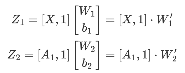
After that, since time-limited, we just tried to add bias to the model we selected (Step size: 0.05, lambda: $10^{−5}$, Hidden layer units: 275, Activation function: Sigmoid), and it got an accuracy of 97.76% in the validation set. It has not shown any huge improvement, maybe because there will be more parameters to train, therefore, it will take longer to train. But it is hard to say whether it will generate an even better model. So, we should try it if time permitting.

If you want to try the model with bias, you can just follow the instruction written in file "train_find_hp.py" and "test_model.py".