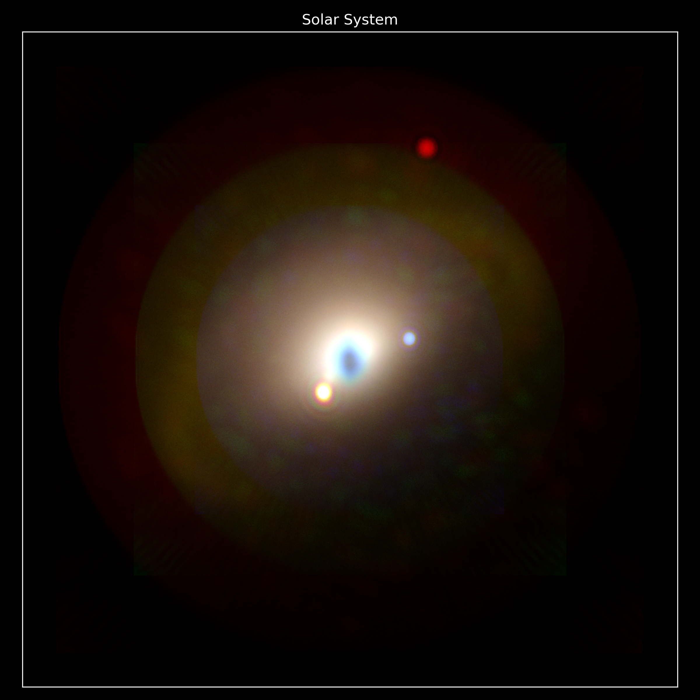
---

coronagraphoto

coronagraphoto is a Python library designed to simulate coronagraphic observations of exoplanetary systems. The base "thing" it produces are images/photos, hence the name. It has been designed to bridge the gap between yield calculations and concrete image generation for missions like the Habitable Worlds Observatory (HWO).

The library integrates high-fidelity coronagraph models from the standard format used for yield calculations (dubbed a "Yield Input Package" and loaded via yippy) with detailed planetary system simulations (via ExoVista) to produce realistic detector images.

Built on JAX, coronagraphoto is fully JIT-compilable, differentiable, and GPU-accelerated, making it suitable for large-scale optimization and high-performance simulation.

Key Features

• End-to-End Simulation: From astrophysical scenes to detector readouts.
• JAX & JIT Compatible: High-performance simulations using functional programming patterns.
• Modular Design: flexible optical paths, easily swappable coronagraphs and detectors.
• HWO Ready: Specifically designed to support yield modeling for future direct imaging missions.

Installation

pip install coronagraphoto

(Note: You may need to install JAX separately to match your specific hardware acceleration requirements (CUDA/TPU/CPU).)

Design philosophy: "Bring your own physics"

coronagraphoto does not provide a single, black-box run_simulation() function. It provides per-source simulation functions and a thin orchestrator that sums them. Scene primitives (Star, Planet, Disk, System, Scene, backgrounds) live in skyscapes, and hardware primitives (OpticalPath, primaries, detectors, throughput elements) live in optixstuff. The convention:

• Noiseless rates: <source>_rate(source, optical_path, *, observation_kwargs) returns the deterministic photo-electron rate map (electrons/s/pixel) for one source. These are differentiable, so they serve as the forward model for fitting and retrievals.
• Noisy readouts: <source>_readout(source, optical_path, prng_key, *, observation_kwargs) adds photon Poisson and quantum-efficiency noise to produce one detector readout.
• Whole-scene orchestrators: system_rate(scene, optical_path, *, ...) and system_readout(scene, optical_path, prng_key, *, ...) sum the star, every planet, the optional disk, the optional zodi, and the optional speckle field from a skyscapes.Scene.

This keeps the pipeline transparent (you know exactly which sources contributed), flexible (drop in custom noise, return spectral cubes, difference two scenes), and fast (each per-source kernel is JIT-cached at its natural shape boundary).

Quick start

import jax
from optixstuff import ConstantThroughput, IdealDetector, OpticalPath, SimplePrimary
from yippy import EqxCoronagraph

from coronagraphoto import load_scene_from_exovista, system_readout
from coronagraphoto.datasets import fetch_coronagraph, fetch_scene

# 1. Load a skyscapes.Scene (system + default zodi) from an ExoVista file.
#    load_disk=False because this example skips the PSF datacube the disk
#    pipeline would need (set ensure_psf_datacube=True and drop the flag
#    to render the disk too).
scene = load_scene_from_exovista(fetch_scene(), load_disk=False)

# 2. Build the optical path from optixstuff hardware primitives + a yippy coronagraph.
coronagraph = EqxCoronagraph(fetch_coronagraph(), ensure_psf_datacube=False)
optical_path = OpticalPath(
    primary=SimplePrimary(diameter_m=6.0),
    attenuating_elements=(ConstantThroughput(throughput=0.9),),
    coronagraph=coronagraph,
    detector=IdealDetector(pixel_scale_arcsec=0.01, shape=coronagraph.psf_shape),
)

# 3. Simulate one detector readout. The epoch must lie inside the ExoVista
#    file's time grid (this demo scene covers JD 2451544.5 to 2455205.0);
#    epochs outside the grid return NaN flux.
image = system_readout(
    scene,
    optical_path,
    jax.random.PRNGKey(0),
    start_time_jd=2_452_000.0,
    exposure_time_s=3600.0,
    wavelength_nm=550.0,
    bin_width_nm=50.0,
    telescope_pa_deg=0.0,
    ecliptic_lat_deg=0.0,
    solar_lon_deg=135.0,
)

# Or the noiseless, differentiable forward model of the same scene:
from coronagraphoto import system_rate

rate = system_rate(
    scene,
    optical_path,
    start_time_jd=2_452_000.0,
    wavelength_nm=550.0,
    bin_width_nm=50.0,
    telescope_pa_deg=0.0,
    ecliptic_lat_deg=0.0,
    solar_lon_deg=135.0,
)

For broadband / IFS simulations, jax.vmap over wavelength_nm (and sum or stack the result) -- the kwarg-only signature is designed so the wavelength axis is a clean vmap target.

Speckles

Time-varying residual-speckle fields plug in through OpticalPath.speckle (any optixstuff.AbstractSpeckleField). When set, system_rate / system_readout add the speckle contribution automatically: the field's realize(wavelength_nm=..., time_s=...) contrast map is multiplied by the host-star flux and resampled to the detector, with evolution driven deterministically by time so that temporal correlation survives across a roll sequence.