{% include mathjax.html %}
Wikipedia is a rich source of human-readable information on a vast variety of subjects. Automatic extraction of its content should prove useful for many data related projects. We aim to extract insights from Wikipedia articles on people (David Bowie, etc.) using natural language processing (NLP) techniques.
We hope, at least, to be able to classify a person into distinct categories (extracted, perhaps, using tf-idf) based on the content of his/her Wikipedia article. For example, the topics extracted from the database using Latent Dirichlet Allocation should give insights on ways to classify a person. We want to be able to tell, for example, based on the topic distributions if the person described in a Wikipedia article is a politician, an artist, or a singer, etc.
As probability vectors, LDA distributions also give us embeddings into high-dimensional space from which we can find embeddings into 2 or 3 dimensions for visualization. Then, if time permits, we may also learn to generate fake Wikipedia articles using Markov models and GANs.
Wikipedia put articles about people with listed birthdates into a list here. Scraping pages off it gives us a huge collection of links, 1.37 million in total, to Wikipedia articles about people. One million is hardly a big number when it comes to data science. But it is a big number for the collective memory. Humanity really only remembers the big blots in its history like Shakespeare or Hitler or Napoléon, and stars that just went out like Stephen Hawking. There are not a million people like those. To sift away the forgotten, we ask Wikipedia for page views which can be done by making a million requests like this one we made for Mister Rogers. These numbers tell us where the limelight shines.
| Rank | Name | Views |
|---|---|---|
| 1 | Louis Tomlinson | 32647670 |
| 2 | Freddie Mercury | 22261530 |
| 3 | Elizabeth II | 20049022 |
| 4 | Stephen Hawking | 19025060 |
| 5 | Donald Trump | 18663083 |
| 6 | Cristiano Ronaldo | 18467102 |
| 7 | Cardi B | 17955598 |
| 8 | Elon Musk | 17836456 |
| 9 | XXXTentacion | 15249774 |
| 10 | Lionel Messi | 13457818 |
| 11 | LeBron James | 12555210 |
| 12 | Ariana Grande | 12307383 |
| 13 | Jason Momoa | 12208869 |
| 14 | 6ix9ine | 12091008 |
| 15 | George H.W. Bush | 12078037 |
| 16 | Anthony Bourdain | 11867794 |
| 17 | Priyanka Chopra | 11613801 |
| 18 | John McCain | 11550433 |
| 19 | Queen Victoria | 11415901 |
| 20 | Stan Lee | 11352622 |
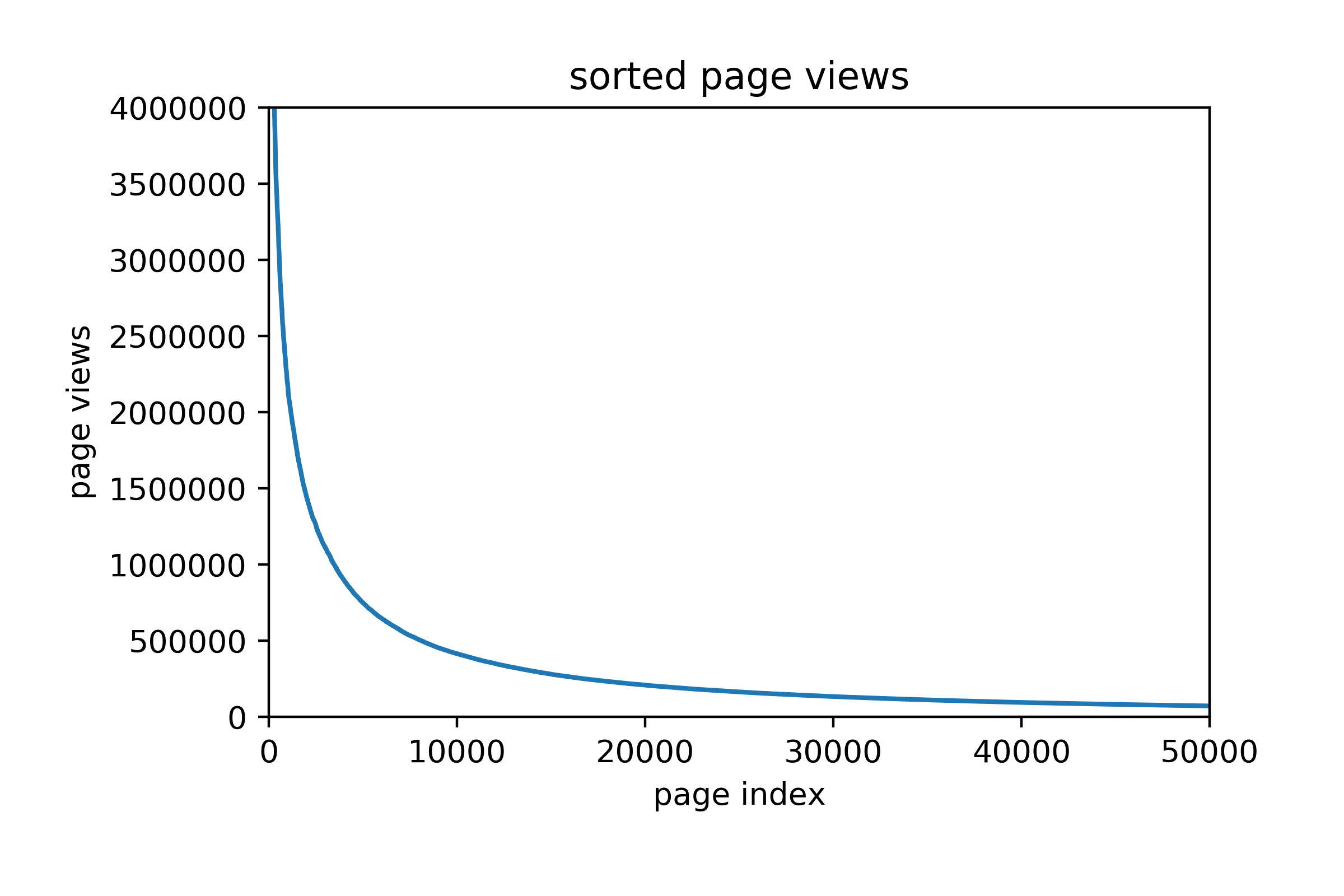
For those who asked the same question we did (with or without expletives), Louis Tomlinson is a member of One Direction. How he came to have 15 times more page views than his other band members remains a mystery beyond the reach of our intelligence. Taking data as fact, sorting the page views in decreasing order gives us the graph below showing a rapidly decaying number of views as you fall down the popularity ladder.
We took the
- Articles with more views are better maintained, and
- Most people don't care about the rest.
In addition to graciously providing views statistics, Wikipedia's API endpoint also extracts plaintext from Wikipedia markup language when asked nicely. At this point, we know who we want in our dataset, the link to their page, and how to extract plaintext from it, collecting data is simply a matter of waiting for page requests.
Now, it has never been a matter of debate that the most insightful part of a Wikipedia article is the so-called lead. In our case, the lead section tells us what the person does, what they are known for and, in general, why they deserve a Wikipedia article. So for most of the projects in this blog post, we use the stopped-tokenized-lemmatized bag-of-words representation of the lead section.
Altogether, the
The main insight of tf-idf is that important words should give information about the articles containing them. In particular, they should appear rather frequently in documents that contain them, but not so ubiquitously that they show up in every other article. The simplest of the tf-idf formulae articulating this train of thought is
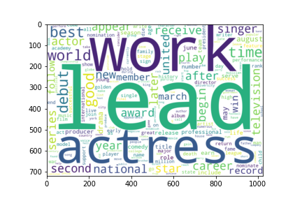
Using the tf-idf formula above to rank the words gives us an expected result, which we show in the wordcloud below.
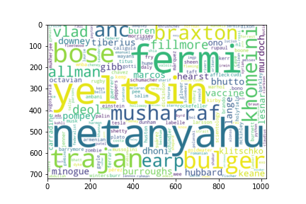
We can see the the most important words are names, which makes sense because important words should distinguish between articles. But not very interesting because we already know that these words are important. To counteract this phenomenon, we only consider common English words, i.e., words you would see in an English dictionary. This leaves us with 3815 unique words, the wordcloud of whose is shown below.
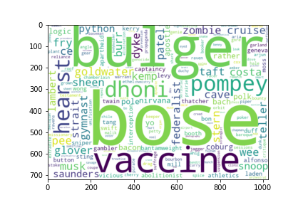
Words like "cave" and "pompey" and "vaccine" definitely tell us a lot about the articles containing them, but they don't cover enough of the corpus to give us a big picture. (If you read on, you will see that over half of the articles are about actors or actresses, but it's impossible to tell just looking at these words that there are any famous actors.) Upon closer inspection, these words only appear in very few documents, so their idf-weights are very high despite not appearing a lot. We experimented with other tf-idf formulae:
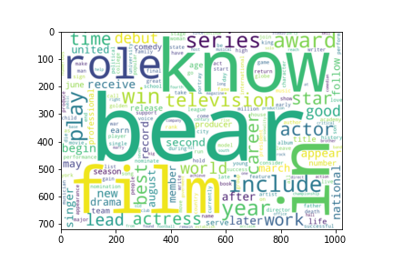
After a few different experiment with weighting, we ended up with a method to calculate idf which wikipedia calls probabilistic idf.
where
From 10,000 most viewed Wikipedia pages in People category, 9,620 pages has 'Categories' property that can be accessed by requesting to Wikipedia API.
To illustrate, Wikipedia has 'Michael Jackson' fit the following categories: '1958 births', '2009 deaths', '20th-century American singers', '21st-century American singers', 'AC with 15 elements', 'Accidental deaths in California', 'African-American choreographers', 'African-American dancers', 'African-American male dancers', 'African-American male singers'
Since 'Categories' property summarizes each person and focus on their occupations, nationalities, and ethnicities, we hope that we can classify people into groups using their categories already made by Wikipedia.
Firstly, we tried Nearest Neighbor Search to find the closest match of each person. In the data preparation process, we discard categories that do not relate to the person's identity. Those categories commonly contains the words 'articles', 'pages', etc. Then, we use a one-hot encoding i.e. dummy variable to convert categories into integer data. After the preparation, we have sklearn.NearestNeighbor fit the one-hot data and predict top two closest match of each person.
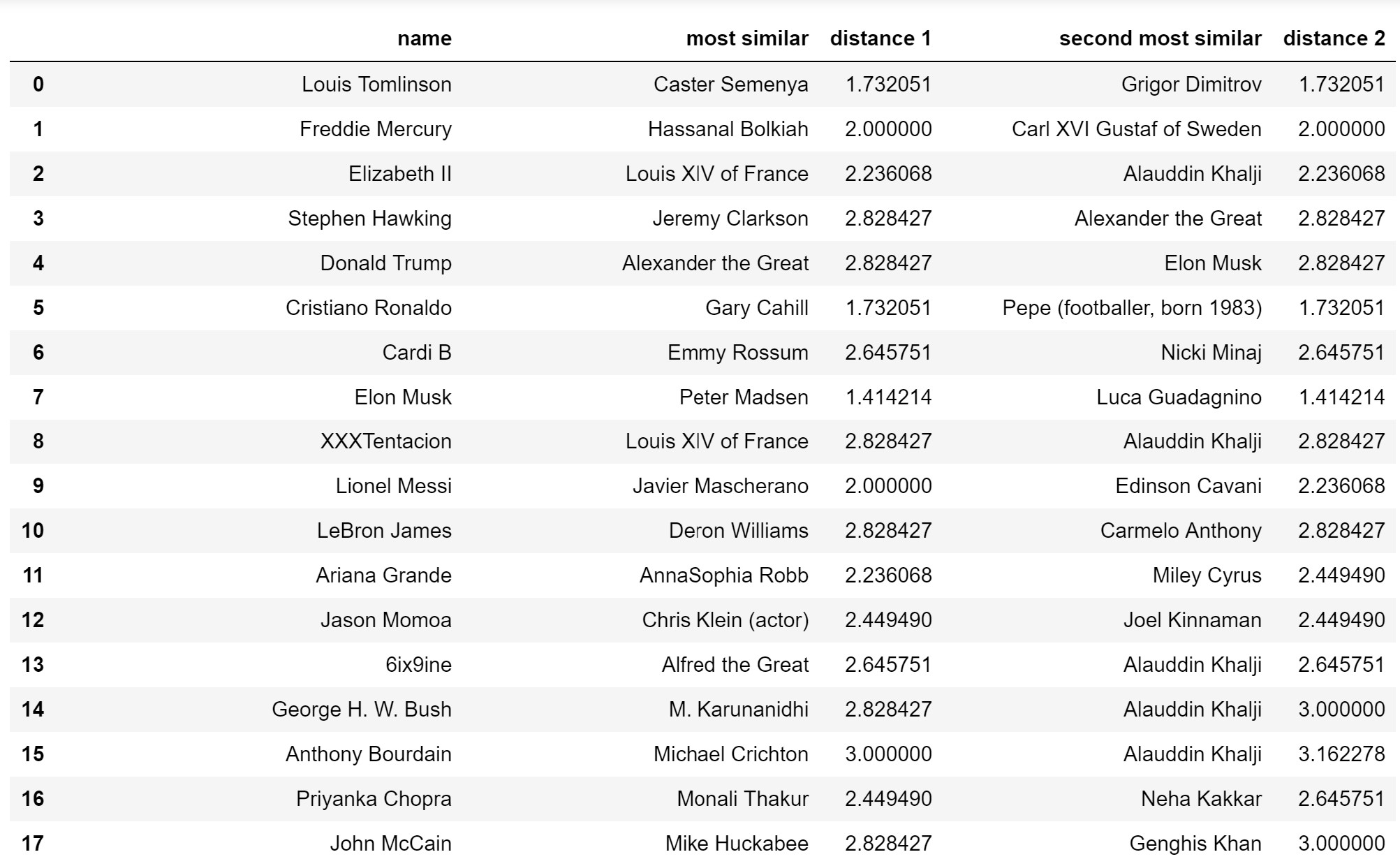
In the first try, we have a dummy variable for every category that appears more than 7 times. The predictions of the 17 most viewed Wikipedia pages are as follow.
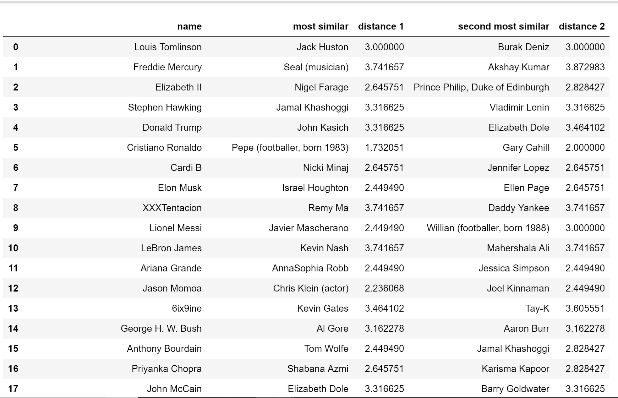
To improve the predictions, we tokenize the categories and have important words representing each person instead. This is because we can create subcategories from the categories given by Wikipedia. For instance, with tokenized version, Michal Jackson will belong to 'American', 'Africa-American', 'dancers', 'singers', etc. Without the tokenization, Michael Jackson would never be matched to an American dancer even though they are similar.
Thus, we tokenize importanct categories and perform Nearest Neighbor Search with the new one-hot matrix. The predictions from this try is more accurate.
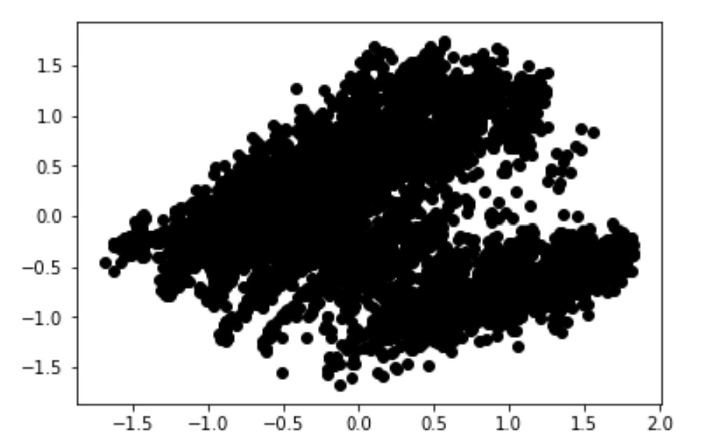
We also plotted this one-hot of tokenized categories hoping for distinct clusterings. The graph is shown below.
We might be able to improve Nearest Neighbor Search by adding weights to similar words. Apart from NNS, we plan to use the categories property provided by Wikipedia to classify people into groups. Possibly, we can present common features of pages that have high views by exploring the categories.
We also experimented with document clustering. We first turn Wikipedia pages to numeric representations using doc2vec. doc2vec is a modified word2vec algorithm, designed to capture semantic information of a document. As an addition to word2vec, a document ID is concatenated to the input word sequence. The learned embedding of each document ID is the vector representation of the document.
Once we obtain the representations of all the documents, we utilize the k-means algorithm to cluster the documents. We ran doc2vec and k-means on the dataset of 10,000 Wikipedia pages. Setting the number of clusters to 10, we obtained the following results with doc2vec.
| Cluster | Word Cloud | Example | Number of Pages | Variance |
|---|---|---|---|---|
| 1 | 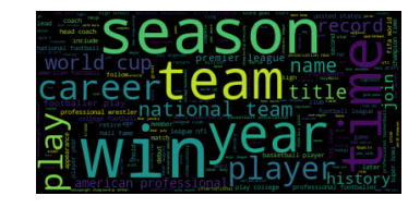 |
LeBron James, Dwayne Johnson, Tonya Harding, Khabib Nurmagomedov, John Cena, Stephen Curry, Anthony Joshua, Caitlyn Jenner, Naomi Osaka, The Undertaker | 814 | 0.0188 |
| 2 | 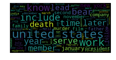 |
Anthony Bourdain, Meghan, Duchess of Sussex, Charles, Prince of Wales, Prince Philip, Duke of Edinburgh, Pablo Escobar, Jeff Bezos, Diana, Princess of Wales, Prince William, Duke of Cambridge, Jeffrey Dahmer, Prince Harry, Duke of Sussex | 956 | 0.0188 |
| 3 | 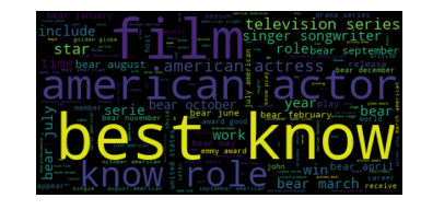 |
Louis Tomlinson, Antonio Maria Magro, Dua Lipa, Pete Davidson, Andrew Cunanan, Hailey Baldwin, Dolores O'Riordan, John Paul Getty III, Lisa Bonet, Beto O'Rourke | 3597 | 0.0055 |
| 4 | 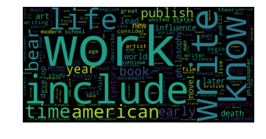 |
Elon Musk, Stephen Hawking, P. T. Barnum, Albert Einstein, Ted Kaczynski, Steve Jobs, William Shakespeare, Bill Gates, Rajneesh, Nikola Tesla | 342 | 0.0322 |
| 5 | 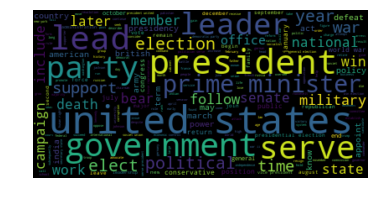 |
Donald Trump, George H. W. Bush, John McCain, Winston Churchill, Barack Obama, Adolf Hitler, Brett Kavanaugh, Mahatma Gandhi, George W. Bush, Martin Luther King Jr. | 336 | 0.0429 |
| 6 | 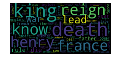 |
Elizabeth II, Queen Victoria, Princess Margaret, Countess of Snowdon, George VI, Mary, Queen of Scots, Edward VIII, George V, Elizabeth I of England, Joaquín "El Chapo" Guzmán, Henry VIII of England | 253 | 0.0428 |
| 7 | 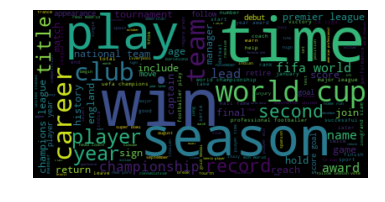 |
Cristiano Ronaldo, Lionel Messi, Michael Jordan, Tom Brady, Kylian Mbappé, Mohamed Salah, Conor McGregor, Roger Federer, Virat Kohli, Neymar | 387 | 0.0414 |
| 8 | 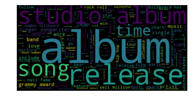 |
Cardi B, Freddie Mercury, XXXTentacion, Ariana Grande, 6ix9ine, Avicii, Donald Glover, Nick Jonas, Post Malone, Michael Jackson | 697 | 0.0269 |
| 9 | 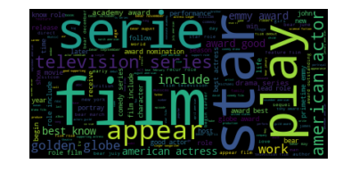 |
Jason Momoa, Stan Lee, Sylvester Stallone, Jennifer Aniston, Michael B. Jordan, Burt Reynolds, Ryan Reynolds, Chris Hemsworth, Josh Brolin, Gianni Versace | 1930 | 0.0106 |
| 10 | 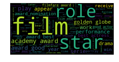 |
Priyanka Chopra, Sridevi, Tom Cruise, Demi Lovato, Clint Eastwood, Scarlett Johansson, Emily Blunt, Keanu Reeves, Bradley Cooper, John Krasinski | 688 | 0.0247 |
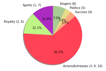
Clustering allows us to better understand out dataset. From the table, we see that there are 6 main "categories" in our dataset: (1) sports (Clusters 1, 7), (2) royalty (Clusters 2, 6), (3) actors/actesses, movies-related figures (Clusters 3, 9, 10), (4) successful figures (Cluster 4), (5) politic figures (Cluster 5), and (6) singers (Cluster 8). From the wordclouds, we also see that the important words are corresponding to each cluster. For instance, the word "work" was extracted as the most important word in Cluster 4, which represent those best known for their career successes such as Elon Musk, Albert Einstein and William Shakespeare. Moreover, we notice that the dataset is highly imbalanced as shown in the chart below. More than half of the dataset are actors/actresses or movies-related figures, while only 3% are political figures.
However, there are some issues concerning our clustering. The first issue is a trade off between a large and small numbers of clusters. When we have too many clusters, some categories might be duplicated or very similar as the results we obtained when having 10 clusters. On the other hand, when we have a small number of clusters, a cluster may include irrelevant pages. As an example, Anthony Bourdain who was a chef was put in the royal families cluster (Cluster 2). While solving the trade off problem is not trivial, a possible work around for this is using alternative embeddings which better represent information about each cluster. As an idea, if we want to cluster documents based on occupations, we can build a neural network which enbeds documents and is trained to predict occupations.