English | 中文

StatsPAI: The Agent-Native Causal Inference & Econometrics Toolkit for Python

StatsPAI is the agent-native Python package for causal inference and applied econometrics. One import, 800+ functions, covering the complete empirical research workflow — from classical econometrics to cutting-edge ML/AI causal methods to publication-ready tables in Word, Excel, and LaTeX.

Designed for AI agents: every function returns structured result objects with self-describing schemas (list_functions(), describe_function(), function_schema()), making StatsPAI the first econometrics toolkit purpose-built for LLM-driven research workflows — while remaining fully ergonomic for human researchers.

It brings R's Causal Inference Task View (fixest, did, rdrobust, gsynth, DoubleML, MatchIt, CausalImpact, ...) and Stata's core econometrics commands into a single, consistent Python API.

---

Quick Start — 60 seconds

pip install statspai, then run any of the four canonical causal-inference exercises below. StatsPAI ships the classic teaching datasets bundled under sp.datasets — Callaway–Sant'Anna mpdta, Card (1995) returns-to-schooling, Abadie–Diamond–Hainmueller California Prop 99, Lee (2008) Senate RD, LaLonde / NSW–DW, Angrist–Krueger (1991) QOB, Basque terrorism, German reunification — so every snippet runs offline with no data wrangling.

import statspai as sp

sp.datasets.list_datasets()   # name / design / n_obs / paper / expected_main

DiD — Callaway & Sant'Anna staggered ATT on mpdta

Minimum-wage effect on teen employment (the canonical example used in R's did package).

import statspai as sp

df = sp.datasets.mpdta()
cs = sp.callaway_santanna(data=df, y='lemp', t='year',
                          i='countyreal', g='first_treat')
print(sp.aggte(cs, type='simple').summary())
# Simple ATT ≈ -0.033, bootstrap SE ≈ 0.004, p < 0.001

IV — Card (1995) returns to schooling

Instrument endogenous educ with proximity to a 4-year college (nearc4).

import statspai as sp

df = sp.datasets.card_1995()
iv = sp.ivreg('lwage ~ (educ ~ nearc4) + exper + expersq + black + south + smsa',
              data=df)
print(iv.summary())
# educ coefficient ≈ 0.142 (SE 0.019); first-stage F ≈ 160; Hausman p ≈ 0.03

RD — Lee (2008) incumbent advantage

Sharp RD around the 0-margin cutoff with Calonico–Cattaneo–Titiunik robust bias-corrected inference.

import statspai as sp

df = sp.datasets.lee_2008_senate()
rd = sp.rdrobust(data=df, y='voteshare_next', x='margin', c=0)
print(rd.summary())
# RD estimate ≈ 0.062 (SE 0.024) — incumbent advantage in next-term voteshare

Synthetic Control — California Proposition 99

Abadie, Diamond & Hainmueller's canonical tobacco-policy evaluation.

import statspai as sp

df = sp.datasets.california_prop99()
sc = sp.synth(data=df, outcome='cigsale', unit='state', time='year',
              treated_unit='California', treatment_time=1989)
print(sc.summary())
# Post-1988 ATT ≈ -13.3 packs/capita

What each result object gives you for free

Beyond the point estimate, every .summary() above prints inference scaffolding you would otherwise hand-assemble from 3–4 separate R packages:

• DiD — aggte[simple] carries a uniform critical value (1.96), balanced_e / min_e / max_e event-time bookkeeping, and 1 000-replication multiplier-bootstrap SEs.
• IV — Partial R²(educ) ≈ 0.051 and first-stage F ≈ 160 (comfortably above Stock–Yogo's rule-of-thumb 10), so weak-instrument risk is visible without a second call.
• RD — Conventional (0.073) and Robust bias-corrected (0.062) estimators print side-by-side with effective-sample counts (440 left / 443 right) at the mserd bandwidth.
• Synth — full 12-period treated-vs-counterfactual gap table; ridge_lambda ≈ 112.9 flags that the ASCM (Ben-Michael, Feller & Rothstein 2021) branch is active. Pass method='adh' to fall back to classical Abadie–Diamond–Hainmueller (ATT ≈ -13.1 on the same panel).

Every result object exposes the same interface — .summary() / .tidy() / .plot() / .to_latex() / .to_docx() / .to_agent_summary() — across all 800+ estimators. For deeper walkthroughs (staggered DiD, weak-IV diagnostics, RD bandwidth choice, 20 synth methods, DML, matching, spatial, ...) see docs/guides/.

---

📊 Causal Inference Coverage at a Glance

StatsPAI's focus is causal inference — and on this axis we aim to be the most complete single package in any language. "Stata" = official + major SSC packages. "R" = CRAN. "sm+lm" = statsmodels + linearmodels.

Method family	Stata	R	sm+lm	DoubleML	StatsPAI
DiD — staggered (CS/SA/BJS/dCdH/Gardner/Wooldridge ET) + event-study + honest CIs	⚠️	✅	❌	❌	🏆
IV — classical (2SLS/LIML/GMM) + modern (Kernel IV / Deep IV / KAN-DeepIV)	✅ classical only	✅ classical only	⚠️ classical	⚠️	🏆
RD — CCT + 2D / boundary + multi-cutoff + honest CIs + ML-CATE (18+ estimators)	⚠️	✅ (rdrobust)	❌	❌	🏆
Synthetic Control — ADH / ASCM / gsynth / BSTS / Bayesian / PenSCM / FDID (20 methods)	⚠️	⚠️ (7 pkgs)	❌	❌	🏆
Double / Debiased ML	❌	✅	❌	✅	✅
Meta-Learners (S/T/X/R/DR) + Causal Forest / GRF	❌	✅	❌	❌	✅
TMLE / HAL-TMLE	❌	✅	❌	❌	✅
Neural causal (TARNet / CFRNet / DragonNet)	❌	❌	❌	❌	🏆
Causal discovery (NOTEARS / PC / LiNGAM / GES)	❌	⚠️	❌	❌	🏆
Proximal CI (fortified / bidirectional / MTP / DNC)	❌	⚠️	❌	❌	🏆
QTE / distributional TE / CiC / dist-IV	⚠️	⚠️	❌	❌	✅
Mendelian randomization (IVW/Egger/median/mode/PRESSO/MVMR/BMA)	❌	✅	❌	❌	✅
Conformal causal inference	❌	❌	❌	❌	🏆
Bayesian Causal Forest (BCF / ordinal / factor-exposure)	❌	⚠️	❌	❌	✅
Spatial econometrics (weights → ESDA → ML/GMM → GWR/MGWR → panel)	❌	⚠️ (5 pkgs)	❌	❌	🏆

Legend: 🏆 most complete across ecosystems · ✅ full coverage · ⚠️ partial / scattered / single algorithm · ❌ not available.

StatsPAI at a glance: 889 registered functions · 78 modules · 188,244 LOC (core) + 42,768 LOC (tests). For the full coverage matrix (23 method families), per-module breakdown, and cross-ecosystem line-count comparison — see docs/stats.md.

---

🎉 NEW in v1.6.0 — P1 Agent-Native × Frontier (LLM-DAG + sp.paper() + Causal-Text + MR frontier + long-panel DML + agent-native infrastructure)

StatsPAI 1.6.0 is a pure-additive minor release pushing two competitive axes simultaneously: agent-native adoption (closed-loop LLM-DAG, end-to-end publication pipeline, 30 populated agent cards, typed exception taxonomy with recovery hints, auto-generated ## For Agents blocks in every flagship guide) and the methodological frontier (five post-2020 Mendelian-randomization estimators, long-panel Double-ML, constrained PC discovery, two causal_text MVPs).

Area	v1.6 Highlights
Agent-native pipeline	sp.paper(data, question, ...) — orchestrator on top of sp.causal() that parses a natural-language question, runs diagnose → recommend → estimate → robustness, and assembles a 7-section PaperDraft (Question / Data / Identification / Estimator / Results / Robustness / References) with .to_markdown() / .to_tex() / .to_docx() / .write(path). Per-section failure isolation: a failed estimator yields a "Pipeline notes" section rather than crashing the draft. Family guide: docs/guides/paper_pipeline.md.
LLM × DAG (closed-loop)	sp.llm_dag_constrained — iterate propose → constrained PC → CI-test validate → demote until convergence. Every kept edge carries llm_score + ci_pvalue + source ∈ {required, forbidden, demoted, ci-test}. result.to_dag() round-trips into statspai.dag.DAG. sp.llm_dag_validate audits any declared DAG edge-by-edge for spuriousness. sp.pc_algorithm(forbidden=, required=) injects background knowledge into PC (default None preserves prior contract). Family guide: docs/guides/llm_dag_family.md.
Causal × Text (experimental)	sp.text_treatment_effect — Veitch-Wang-Blei (2020 UAI) text-as-treatment ATE via embedding-projected OLS with HC1 SEs; hash embedder default (deterministic, dependency-free), lazy sbert optional. sp.llm_annotator_correct — Egami-Hinck-Stewart-Wei (2024) Hausman-style measurement-error correction for binary LLM-derived treatments; raises IdentificationFailure when the LLM has no information. Both subclass CausalResult and ship full agent-card metadata. Family guide: docs/guides/causal_text_family.md.
MR frontier (5 new)	sp.mr_lap (Burgess-Davies-Thompson 2016 sample-overlap-corrected IVW). sp.mr_clust (Foley-Mason-Kirk-Burgess 2021 clustered MR via finite Gaussian mixture on Wald ratios, BIC-selected K). sp.grapple (Wang-Zhao-Bowden-Hemani 2021 profile-likelihood MR with joint weak-instrument + balanced-pleiotropy robustness). sp.mr_cml (Xue-Shen-Pan 2021 constrained maximum-likelihood MR with L0-sparse pleiotropy, MR-cML-BIC). sp.mr_raps (Zhao-Wang-Hemani-Bowden-Small 2020 Annals of Statistics robust adjusted profile score with Tukey biweight loss). sp.mr(method='lap' | 'clust' | 'grapple' | 'cml' | 'raps') dispatcher routes all five. 41 new tests in tests/test_mr_frontier.py.
Long-panel Double-ML	sp.dml_panel — Semenova-Chernozhukov (2023) long-panel DML: absorbs unit (+ optional time) fixed effects via within-transform, cross-fits ML nuisance learners with unit-split folds (Liang-Zeger compatible), reports cluster-robust SE at the unit level. Empty-covariate fallback reduces to pure FE-OLS. 13 new tests.
Typed exception taxonomy	StatsPAIError root + AssumptionViolation / IdentificationFailure / DataInsufficient / ConvergenceFailure / NumericalInstability / MethodIncompatibility, each carrying recovery_hint, machine-readable diagnostics, and a ranked alternative_functions list. Warning counterparts: StatsPAIWarning / ConvergenceWarning / AssumptionWarning plus a rich-payload sp.exceptions.warn() helper. Domain errors subclass ValueError / RuntimeError → existing except blocks keep working unchanged. 13 call-site migrations already shipped (DID, IV, matching, DML-IRM, synth, Bayesian DML).
Agent cards + registry	sp.agent_card(name) and sp.agent_cards(category=None) return pre_conditions / assumptions / failure_modes (symptom + exception + remedy + alternative) / alternatives / typical_n_min for 36 flagship functions (regress, iv, did, callaway_santanna, rdrobust, synth, dml, dml_panel, causal_forest, metalearner, match, tmle, bayes_dml, bayes_did, bayes_iv, proximal, mr, qdid, qte, dose_response, spillover, multi_treatment, network_exposure, paper, llm_dag_constrained, llm_dag_validate, text_treatment_effect, llm_annotator_correct, ...). sp.recommend() auto-consumes them: every recommendation now includes agent_card / pre_conditions / failure_modes / alternatives / typical_n_min, with an auto-warning when n_obs < typical_n_min.
Result-object agent hooks	CausalResult.violations() / EconometricResults.violations() inspect stored diagnostics (pre-trend p, first-stage F, McCrary, rhat/ESS/divergences, overlap, SMD) and return flagged items with severity / recovery_hint / alternatives. .to_agent_summary() returns a JSON-ready structured payload (point estimate, coefficients, scalar diagnostics, violations, next-steps) alongside the existing prose .summary() and tidy() DataFrame.
Docs × agents	26 auto-rendered ## For Agents blocks across 19 guides (was 0 pre-v1.5.1) via sp.render_agent_block(name) + scripts/sync_agent_blocks.py (CI-enforced via tests/test_agent_blocks_drift.py). Covers DID / IV / RD / Synth / Matching / DML / Meta-learners / TMLE / Causal-Forest / Bayesian / Proximal / MR / QTE / Interference / Causal-Text / LLM-DAG / Paper-pipeline families.

Every public signature shipped in v1.5.x is byte-for-byte identical in v1.6.0 — this release is purely additive. Existing call sites that catch ValueError continue to catch AssumptionViolation / DataInsufficient / MethodIncompatibility / IdentificationFailure; catching RuntimeError continues to catch ConvergenceFailure / NumericalInstability. New code should prefer the specific subclasses and attach a recovery_hint so agents can act on failures without parsing error strings.

Previously in v1.5.0 — Interference / Conformal / Mendelian family consolidation

StatsPAI 1.5.0 was a minor release bundling three concurrent improvements to the interference, conformal causal inference, and Mendelian Randomization families: full-family documentation guides, unified dispatchers matching the sp.synth / sp.decompose / sp.dml pattern, and a targeted correctness audit that fixed two silent-wrong-numbers issues.

• Family guides (3 new) — docs/guides/interference_family.md (9 estimators + decision tree + 5 diagnostics), docs/guides/conformal_family.md (all 10 conformal estimators organised around marginal-coverage guarantee), docs/guides/mendelian_family.md (17 MR functions by IV1/IV2/IV3 assumption hierarchy + worked BMI → T2D example).
• Unified dispatchers (3 new) — sp.mr(method=...) (33 aliases), sp.conformal(kind=...) (29 aliases), sp.interference(design=...) (29 aliases). Byte-for-byte identical to direct calls (30 parity tests guarantee this).
• ⚠️ Correctness — sp.mr_egger: slope inference fixed to t(n−2) (was stats.norm). Anti-conservative at small n_snps; numerically invisible for n_snps ≥ ~100.
• ⚠️ Correctness — sp.mr_presso: MC p-value switched from raw mean(null ≥ obs) to standard (k+1)/(B+1) convention (matches R's MR-PRESSO). No longer silently produces -inf.
• ⚠️ Breaking — sp.mr module → function dispatcher. Module access preserved at sp.mendelian. See MIGRATION.md.

Previously in v1.4.2 — correctness patches + Proximal / QTE / Causal-RL family guides

StatsPAI 1.4.2 was a patch release with two silent-wrong-numbers fixes and three family guides:

• ⚠️ correctness fix — sp.dml_model_averaging √n SE scaling bug. The cross-candidate variance aggregator treated the sample-mean influence-function outer product as Var(θ̂_avg) directly, missing a final / n. Reported SEs were √n times too large; on the canonical n=400 DGP the 95% CI width was 4.20 (nominal ≈ 0.21) and empirical coverage was 100%. After the fix, CI width is 0.21 and coverage is ≈ nominal. Regression guard: tests/test_dml_model_averaging.py::test_se_on_correct_scale.
• ⚠️ correctness fix — sp.gardner_did event-study reference-category contamination. Stage-2 dummy regression pooled never-treated units and treated units outside the event-study horizon into a single baseline, dragging every event-time coefficient toward the mean of that pool. On a synthetic panel with true τ=2 and strict parallel trends, pre-trends came out ≈ -0.30 (should be 0) and post ≈ +1.72 (should be 2.0). Replaced the Stage-2 regression in event-study mode with direct Borusyak-Jaravel-Spiess-style within-(cohort × relative-time) averaging of the imputed gap. After the fix: pre-trends ≈ +0.01, post ≈ +2.02. Non-event-study single-ATT path was already correct and is unchanged.
• Family guides — docs/guides/proximal_family.md (full Proximal Causal Inference walkthrough), docs/guides/qte_family.md (mean → quantile → distribution), docs/guides/causal_rl_family.md (causal RL vs classical CI).
• Formally shipped from v1.4.1 cherry-picks — tests/test_bridge_full.py (10 end-to-end tests for sp.bridge(kind=...) bridging theorems) and docs/guides/bridging_theorems.md.

Previously in v1.4.1 — v3-frontier Sprint 3: AKM shock-clustered SE, Claude extended thinking, parity + integration suites, 2 new guides

StatsPAI 1.4.1 is an additive follow-up to 1.4.0 that closes the Sprint 3 items:

• AKM shock-clustered SE — sp.shift_share_political_panel(cluster='shock') computes the panel-extended Adão-Kolesár-Morales (2019) variance estimator recommended by Park-Xu (2026) §4.2 — typically 3× tighter than unit-clustered SEs in settings with 10–100 industries. diagnostics['akm_se'] and a human-readable diagnostics['cluster'] label surface the result.
• Claude extended thinking for Causal MAS — sp.causal_llm.anthropic_client(thinking_budget=N) opts into the Claude 4.5 / Opus 4.7 extended-thinking API. The reasoning trace is captured on client.history[-1]['thinking'] for auditability but is not returned to causal_mas. Handles both thinking and redacted_thinking content blocks.
• Parity + integration test suites — tests/reference_parity/test_assimilation_parity.py (10 checks on the Kalman / particle backends, incl. Kalman↔particle agreement and Student-t contamination robustness) and tests/integration/test_causal_mas_with_fake_llm.py (11 end-to-end MAS tests using echo_client + 3 Claude thinking block-splitter tests mocking the Anthropic SDK).
• Two new MkDocs guides — docs/guides/shift_share_political_panel.md (full panel-IV recipe incl. AKM shock-cluster) and docs/guides/causal_mas.md (multi-agent LLM causal discovery walkthrough).

All v1.4.0 APIs remain stable; the new surface is strictly additive kwargs.

Previously in v1.4.0 — v3-frontier Sprint 2: panel shift-share, real-LLM adapters, particle-filter assimilation, 3 new guides

StatsPAI 1.4.0 is Sprint 2 of the 知识地图 v3 roadmap. Closes the four secondary items flagged at the end of Sprint 1: multi-period Park-Xu political shift-share, real OpenAI / Anthropic LLM adapters for the Causal MAS discovery agent, a particle-filter backend for causal_kalman to handle non-Gaussian priors and nonlinear dynamics, and three new MkDocs guides covering the v3 frontier. 20 unused-import cleanups across Sprint 1 modules. One CI flake (CausalForest ATE parity test) deflaked by seeding the forest explicitly.

Area	v1.4 Highlights
Panel shift-share IV	sp.shift_share_political_panel — Park-Xu (2026) §4.2 multi-period extension: time-varying shares + time-varying shocks, pooled 2SLS with unit / time / two-way FE, per-period event-study table + aggregate Rotemberg top-K. Recovers τ = 0.30 within 0.003 on synthetic 30×4 panels.
Real-LLM adapters (Causal MAS)	sp.causal_llm.openai_client — OpenAI SDK ≥ 1.0 (supports Azure / vLLM / Ollama via base_url). sp.causal_llm.anthropic_client — Anthropic Messages API ≥ 0.30, defaults to claude-opus-4-7. sp.causal_llm.echo_client — deterministic scripted-response client for offline tests. Lazy-imported SDKs → zero new runtime deps on the core package.
Particle-filter assimilation	sp.assimilation.particle_filter — bootstrap-SIR particle filter with systematic resampling (Gordon-Salmond-Smith 1993; Douc-Cappé 2005). Non-Gaussian priors, heavy-tailed observation noise, nonlinear dynamics via pluggable callbacks. Agrees with exact Kalman to ~0.003 under Gaussian DGPs. sp.assimilative_causal(..., backend='particle') routes the end-to-end wrapper.
Documentation (v3 frontier guides)	docs/guides/synth_experimental.md (Abadie-Zhao inverse-SC workflow), docs/guides/harvest_did.md (Borusyak-Hull-Jaravel harvesting DID), docs/guides/assimilative_ci.md (Nature Comms 2026 streaming CI, Kalman + particle backends). Wired into mkdocs.yml nav.
v1.3 stable foundation (carried forward)	11 2025-2026 frontier methods from Sprint 1: synth_experimental_design, rdrobust(..., bootstrap='rbc'), evidence_without_injustice, target_trial.to_paper(fmt='jama'/'bmj'), harvest_did, bcf_ordinal, bcf_factor_exposure, causal_mas, shift_share_political, causal_kalman. All v1.0 capstone surfaces (sp.bridge, sp.fairness, sp.surrogate, sp.epi, sp.longitudinal, sp.question, full MR suite, TARGET checklist) remain intact.
Agent-native platform	sp.list_functions() / sp.describe_function() / sp.function_schema() expose OpenAI/Anthropic tool-calling schemas for 874+ registered estimators. 5 new hand-written FunctionSpec entries this release. sp.agent.mcp_server MCP scaffold lets external LLMs call every StatsPAI function via natural-language tool invocation.
CI/CD hygiene	tabulate hard-dep from v1.3.0 carried forward. Deflaked test_forest_ate_recovers_average_tau by seeding the forest explicitly (random_state=0, n_estimators=300, larger n). 2 699+ tests passing across all OS × Python matrix entries.

Previously in v0.9.2 — Decomposition Analysis: 18 first-class decomposition methods across 13 modules (~6,200 LOC, 54 tests), unified under sp.decompose(method=...). Mean (Blinder-Oaxaca/Gelbach/Fairlie/Bauer-Sinning/Yun), distributional (RIF/FFL/DFL/Machado-Mata/Melly/CFM), inequality (Theil/Atkinson/Dagum/Shapley/Lerman-Yitzhaki), demographic (Kitagawa/Das-Gupta), and causal (gap_closing/mediation_decompose/disparity_decompose). Closed-form influence functions for Theil/Atkinson, weighted O(n log n) Dagum Gini, cross-method consistency checks.

Previously in v0.9.1 — Regression Discontinuity: 18+ RD estimators, diagnostics, and inference methods across 14 modules (~10,300 LOC) — now the most feature-complete RD package in any language. Covers CCT sharp/fuzzy/kink, 2D/boundary RD (rd2d), RDIT, multi-cutoff & multi-score, honest CIs (Armstrong-Kolesar), local randomization (rdrandinf/rdwinselect/rdsensitivity), CJM density tests, Rosenbaum bounds, CATE via rdhte + ML variants (rd_forest/rd_boost/rd_lasso), external-validity extrapolation (Angrist-Rokkanen), power (rdpower/rdsampsi), and a one-click sp.rdsummary() dashboard. 97 RD tests pass; rd/_core.py consolidates kernel/WLS/sandwich primitives from 9 files into one 191-line canonical module.

Previously in v0.9.0 — Synthetic Control: 20 SCM estimators + 6 inference strategies + full research workflow, all behind the unified sp.synth(method=...) dispatcher. Seven new estimators in this release: bayesian_synth (Dirichlet MCMC), bsts_synth / causal_impact (Kalman smoother), penscm (Abadie-L'Hour 2021), fdid (Forward DID), cluster_synth, sparse_synth (LASSO), kernel_synth + kernel_ridge_synth. Research workflow: synth_compare() runs all 20 · synth_recommend() auto-selects · synth_power() + synth_mde() first power-analysis tool for SCM · synth_sensitivity() · synth_report(format='latex'). ASCM re-implemented to Ben-Michael et al. (2021) Eq. 3; Bayesian MCMC Jacobian corrected; 9 release-blocker fixes from a 5-agent review; 144 synth tests passing. Canonical datasets: california_tobacco(), german_reunification(), basque_terrorism(). See the synth guide.

Previously in v0.8.0: Spatial Econometrics Full-Stack — 38 new API symbols covering weights, ESDA, ML/GMM regression, GWR/MGWR, and spatial panel. Plus: local projections, GARCH, ARIMA, BVAR, LiNGAM, GES, optimal matching, cardinality matching, RIF decomposition, mediation sensitivity, Cox frailty, AFT survival, rdpower, survey calibration. 60+ new functions across 10 domains.

Built by the team behind CoPaper.AI · Stanford REAP Program

---

Why StatsPAI?

Pain point	Stata	R	StatsPAI
Scattered packages	One environment, but $695+/yr license	20+ packages with incompatible APIs	One import, unified API
Publication tables	outreg2 (limited formats)	modelsummary (best-in-class)	Word + Excel + LaTeX + HTML in every function
Robustness checks	Manual re-runs	Manual re-runs	spec_curve() + robustness_report() — one call
Heterogeneity analysis	Manual subgroup splits + forest plots	Manual lapply + ggplot	subgroup_analysis() with Wald test
Modern ML causal	Limited (no DML, no causal forest)	Fragmented (DoubleML, grf, SuperLearner separate)	DML, Causal Forest, Meta-Learners, TMLE, DeepIV
Neural causal models	None	None	TARNet, CFRNet, DragonNet
Causal discovery	None	pcalg (complex API)	notears(), pc_algorithm(), lingam(), ges()
Spatial econometrics	None	5 packages (spdep+spatialreg+sphet+splm+GWmodel)	38 functions: weights→ESDA→ML/GMM→GWR/MGWR→panel
Policy learning	None	policytree (standalone)	policy_tree() + policy_value()
Result objects	Inconsistent across commands	Inconsistent across packages	Unified CausalResult with .summary(), .plot(), .to_latex(), .cite()
Interactive plot editing	Graph Editor (no code export)	None	sp.interactive() — GUI editing with auto-generated code

---

What StatsPAI is — and is not

StatsPAI is not a wrapper for R. We independently re-implement every algorithm from the original papers (with citations exposed via .cite()), and for a few mature engines (pyfixest, rdrobust) we use explicit, transparent bindings. What makes StatsPAI different is the unifying layer on top:

• One result object, one API surface. Every estimator — from regress() to callaway_santanna() to causal_forest() to notears() — returns a CausalResult with the same .summary() / .plot() / .to_latex() / .cite() interface. R users juggle 20+ incompatible S3 classes; StatsPAI users juggle one.
• Scope no single R or Python package matches. DID + RD + Synth + Matching + DML + Meta-learners + TMLE + Neural Causal + Causal Discovery + Policy Learning + Conformal + Bunching + Spillover + Matrix Completion — all consistent, all under sp.*.
• Agent-native by design. Self-describing schemas (list_functions(), describe_function(), function_schema()) make StatsPAI the first econometrics toolkit built for LLM-driven research workflows. No other package — in any language — offers this.
• Publication pipeline out of the box. Word + Excel + LaTeX + HTML + Markdown export from every estimator, not a separate modelsummary-style dance.

If a method exists in R, we aim to match or exceed its feature set in Python — and then add what Python can uniquely offer (sklearn integration, JAX/PyTorch backends, agent-native schemas).

---

Complete Feature List

Regression Models

Function	Description	Stata equivalent	R equivalent
regress()	OLS with robust/clustered/HAC SE	reg y x, r / vce(cluster c)	fixest::feols()
ivreg()	IV / 2SLS with first-stage diagnostics	ivregress 2sls	fixest::feols() with IV
panel()	Fixed Effects, Random Effects, Between, FD	xtreg, fe / xtreg, re	plm::plm()
heckman()	Heckman selection model	heckman	sampleSelection::selection()
qreg(), sqreg()	Quantile regression	qreg / sqreg	quantreg::rq()
tobit()	Censored regression (Tobit)	tobit	censReg::censReg()
xtabond()	Arellano-Bond dynamic panel GMM	xtabond	plm::pgmm()
glm()	Generalized Linear Model (6 families × 8 links)	glm	stats::glm()
logit(), probit()	Binary choice with marginal effects	logit / probit	stats::glm(family=binomial)
mlogit()	Multinomial logit	mlogit	nnet::multinom()
ologit(), oprobit()	Ordered logit / probit	ologit / oprobit	MASS::polr()
clogit()	Conditional logit (McFadden)	clogit	survival::clogit()
poisson(), nbreg()	Count data (Poisson, Negative Binomial)	poisson / nbreg	MASS::glm.nb()
ppmlhdfe()	Pseudo-Poisson MLE for gravity models	ppmlhdfe	fixest::fepois()
zip_model(), zinb()	Zero-inflated Poisson / NegBin	zip / zinb	pscl::zeroinfl()
hurdle()	Hurdle (two-part) model	—	pscl::hurdle()
truncreg()	Truncated regression (MLE)	truncreg	truncreg::truncreg()
fracreg()	Fractional response (Papke-Wooldridge)	fracreg	—
betareg()	Beta regression	—	betareg::betareg()
liml()	LIML (robust to weak IV)	ivregress liml	AER::ivreg()
jive()	Jackknife IV (many instruments)	—	—
lasso_iv()	LASSO-selected instruments	—	—
feols()	OLS / IV with high-dim fixed effects (pyfixest backend)	reghdfe	fixest::feols()
fepois()	Poisson with high-dim fixed effects	ppmlhdfe	fixest::fepois()
feglm()	GLM with high-dim fixed effects	—	fixest::feglm()
etable()	Publication-quality regression tables (LaTeX/Markdown/HTML)	esttab	fixest::etable()
sureg()	Seemingly Unrelated Regression	sureg	systemfit::systemfit("SUR")
three_sls()	Three-Stage Least Squares	reg3	systemfit::systemfit("3SLS")
biprobit()	Bivariate probit	biprobit	—
etregress()	Endogenous treatment effects	etregress	—
gmm()	General GMM (arbitrary moments)	gmm	gmm::gmm()
frontier()	Stochastic frontier analysis	frontier	sfa::sfa()

Panel Data (Extended)

Function	Description	Stata equivalent
panel_logit(), panel_probit()	Panel binary (FE conditional / RE / CRE Mundlak)	xtlogit / xtprobit
panel_fgls()	FGLS with heteroskedasticity and AR(1)	xtgls
interactive_fe()	Interactive fixed effects (Bai 2009)	—
panel_unitroot()	Panel unit root (IPS / LLC / Fisher / Hadri)	xtunitroot
mixed()	Linear mixed / multilevel (HLM): unstructured G, 3-level nested, BLUP posterior SEs, Nakagawa–Schielzeth R², caterpillar plot, predict()	mixed
melogit(), mepoisson(), meglm()	Generalised linear mixed models via Laplace approximation (binomial / Poisson / Gaussian) with odds-ratio & IRR tables	melogit / mepoisson / meglm
icc()	Intra-class correlation with delta-method 95% CI	estat icc
lrtest()	Likelihood-ratio test between nested mixed models with Self–Liang χ̄² boundary correction	lrtest

Survival / Duration Analysis

Function	Description	Stata equivalent
cox()	Cox Proportional Hazards	stcox
kaplan_meier()	Kaplan-Meier survival curves	sts graph
survreg()	Parametric AFT (Weibull / exponential / log-normal)	streg
logrank_test()	Log-rank test for group comparison	sts test

Time Series & Cointegration

Function	Description	Stata equivalent
var()	Vector Autoregression	var
granger_causality()	Granger causality test	vargranger
irf()	Impulse response functions	irf graph
structural_break()	Bai-Perron structural break test	estat sbsingle
cusum_test()	CUSUM parameter stability test	—
engle_granger()	Engle-Granger cointegration test	—
johansen()	Johansen cointegration (trace / max-eigenvalue)	vecrank

Nonparametric Methods

Function	Description	Stata equivalent
lpoly()	Local polynomial regression	lpoly
kdensity()	Kernel density estimation	kdensity

Experimental Design & RCT Tools

Function	Description
randomize()	Stratified / cluster / block randomization
balance_check()	Covariate balance with normalized differences
attrition_test()	Differential attrition analysis
attrition_bounds()	Lee / Manski bounds under attrition
optimal_design()	Optimal sample size / cluster design

Missing Data

Function	Description	Stata equivalent
mice()	Multiple Imputation by Chained Equations	mi impute chained
mi_estimate()	Combine estimates via Rubin's rules	mi estimate

Mendelian Randomization

Function	Description
mendelian_randomization()	IVW + MR-Egger + Weighted Median MR
mr_plot()	Scatter plot with MR regression lines

Structural Estimation

Function	Description	Reference
blp()	BLP random-coefficients demand estimation	Berry, Levinsohn & Pakes (1995)

Difference-in-Differences

Function	Description	Reference
did()	Auto-dispatching DID (2×2 or staggered)	—
did_summary()	One-call robustness comparison across CS/SA/BJS/ETWFE/Stacked	—
did_summary_plot()	Forest plot of method-robustness summary	—
did_summary_to_markdown() / _to_latex()	Publication-ready tables from did_summary	—
did_report()	One-call bundle: txt + md + tex + png + json into a folder	—
did_2x2()	Classic two-group, two-period DID	—
callaway_santanna()	Staggered DID with heterogeneous effects	Callaway & Sant'Anna (2021)
sun_abraham()	Interaction-weighted event study	Sun & Abraham (2021)
bacon_decomposition()	TWFE decomposition diagnostic	Goodman-Bacon (2021)
honest_did()	Sensitivity to parallel trends violations	Rambachan & Roth (2023)
continuous_did()	Continuous treatment DID (dose-response)	Callaway, Goodman-Bacon & Sant'Anna (2024)
did_multiplegt()	DID with treatment switching	de Chaisemartin & D'Haultfoeuille (2020)
did_imputation()	Imputation DID estimator	Borusyak, Jaravel & Spiess (2024)
wooldridge_did() / etwfe()	Extended TWFE: xvar= (single/multi) + panel= (repeated CS) + cgroup= (never/notyet)	Wooldridge (2021)
etwfe_emfx()	R etwfe::emfx equivalent — simple/group/event/calendar aggregations	McDermott (2023)
drdid()	Doubly robust 2×2 DID (OR + IPW)	Sant'Anna & Zhao (2020)
stacked_did()	Stacked event-study DID	Cengiz et al. (2019); Baker, Larcker & Wang (2022)
ddd()	Triple-differences (DDD)	Gruber (1994); Olden & Møen (2022)
cic()	Changes-in-changes (quantile DID)	Athey & Imbens (2006)
twfe_decomposition()	Bacon + de Chaisemartin–D'Haultfoeuille weights	Goodman-Bacon (2021); dCDH (2020)
distributional_te()	Distributional treatment effects	Chernozhukov, Fernandez-Val & Melly (2013)
sp.aggte()	Unified aggregation for staggered DID (simple/dynamic/group/calendar) with Mammen multiplier-bootstrap uniform bands	Callaway & Sant'Anna (2021) §4; Mammen (1993)
sp.cs_report()	One-call Callaway–Sant'Anna report: estimation + four aggregations + pre-trend test + Rambachan–Roth breakdown M*	CS2021 + RR2023
sp.ggdid()	aggte() visualiser with uniform-band overlay	mirrors R did::ggdid
CSReport.plot()	2×2 summary figure (event study / θ(g) / θ(t) / RR breakdown)	—
CSReport.to_markdown()	GitHub-Flavoured Markdown export of the full report	—
CSReport.to_latex()	Booktabs LaTeX fragment, jinja2-free	—
CSReport.to_excel()	Six-sheet Excel workbook	—

DiD parity with csdid / differences / R did + HonestDiD

All algorithms below are reimplemented from the original papers — no wrappers, no runtime dependencies on upstream DID packages.

Feature	StatsPAI	csdid (Py)	differences (Py)	R did
Callaway–Sant'Anna ATT(g,t) with DR / IPW / REG	✅	✅	✅	✅
Never-treated / not-yet-treated control group	✅	✅	✅	✅
Anticipation (anticipation=δ)	✅	✅	—	✅
Repeated cross-sections (panel=False)	✅	✅	partial	✅
aggte: simple / dynamic / group / calendar	✅	✅	✅	✅
Mammen multiplier bootstrap, uniform sup-t bands	✅	✅	—	✅
balance_e / min_e / max_e	✅	✅	partial	✅
Sun–Abraham IW with Liang–Zeger cluster SE	✅	—	✅	via fixest::sunab
Borusyak–Jaravel–Spiess imputation + pre-trend Wald	✅	—	—	via didimputation
de Chaisemartin–D'Haultfoeuille switch-on-off	✅	—	—	via DIDmultiplegtDYN
dCDH joint placebo Wald + avg. cumulative effect	✅	—	—	✅ (v2)
Rambachan–Roth sensitivity + breakdown M*	✅	—	—	via HonestDiD
cs ⇄ aggte ⇄ honest_did pipeline (single object)	✅	partial	partial	partial
One-call report card (cs_report)	✅	—	—	via summary()
Markdown / LaTeX / Excel report export	✅	—	—	partial
save_to= one-call bundle (txt + md + tex + xlsx + png)	✅	—	—	—
CSReport.plot() 2×2 summary figure	✅	—	—	—

Regression Discontinuity

Function	Description	Reference
rdrobust()	Sharp/Fuzzy RD with robust bias-corrected inference	Calonico, Cattaneo & Titiunik (2014)
rdplot()	RD visualization with binned scatter	—
rddensity()	McCrary density manipulation test	McCrary (2008)
rdmc()	Multi-cutoff RD	Cattaneo et al. (2024)
rdms()	Geographic / multi-score RD	Keele & Titiunik (2015)
rkd()	Regression Kink Design	Card et al. (2015)

Matching & Reweighting

Function	Description	Stata equivalent
match()	PSM, Mahalanobis, CEM with balance diagnostics	psmatch2 / cem
ebalance()	Entropy balancing	ebalance

Synthetic Control

Function	Description	Reference
synth()	Abadie-Diamond-Hainmueller SCM	Abadie et al. (2010)
sdid()	Synthetic Difference-in-Differences	Arkhangelsky et al. (2021)
Placebo inference, gap plots, weight tables, RMSE plots	—	—

Machine Learning Causal Inference

Function	Description	Reference
dml()	Double/Debiased ML (PLR + IRM) with cross-fitting	Chernozhukov et al. (2018)
causal_forest()	Causal Forest for heterogeneous treatment effects	Wager & Athey (2018)
deepiv()	Deep IV neural network approach	Hartford et al. (2017)
metalearner()	S/T/X/R/DR-Learner for CATE estimation	Kunzel et al. (2019), Kennedy (2023)
tmle()	Targeted Maximum Likelihood Estimation	van der Laan & Rose (2011)
aipw()	Augmented Inverse-Probability Weighting	—

Neural Causal Models

Function	Description	Reference
tarnet()	Treatment-Agnostic Representation Network	Shalit et al. (2017)
cfrnet()	Counterfactual Regression Network	Shalit et al. (2017)
dragonnet()	Dragon Neural Network for CATE	Shi et al. (2019)

Causal Discovery

Function	Description	Reference
notears()	DAG learning via continuous optimization	Zheng et al. (2018)
pc_algorithm()	Constraint-based causal graph learning	Spirtes et al. (2000)

Policy Learning

Function	Description	Reference
policy_tree()	Optimal treatment assignment rules	Athey & Wager (2021)
policy_value()	Policy value evaluation	—

Conformal & Bayesian Causal Inference

Function	Description	Reference
conformal_cate()	Distribution-free prediction intervals for ITE	Lei & Candes (2021)
bcf()	Bayesian Causal Forest (separate mu/tau)	Hahn, Murray & Carvalho (2020)

Dose-Response & Multi-valued Treatment

Function	Description	Reference
dose_response()	Continuous treatment dose-response curve (GPS)	Hirano & Imbens (2004)
multi_treatment()	Multi-valued treatment AIPW	Cattaneo (2010)

Bounds & Partial Identification

Function	Description	Reference
lee_bounds()	Sharp bounds under sample selection	Lee (2009)
manski_bounds()	Worst-case bounds (no assumption / MTR / MTS)	Manski (1990)

Interference & Spillover

Function	Description	Reference
spillover()	Direct + spillover + total effect decomposition	Hudgens & Halloran (2008)

Dynamic Treatment Regimes

Function	Description	Reference
g_estimation()	Multi-stage optimal DTR via G-estimation	Robins (2004)

Bunching & Tax Policy

Function	Description	Reference
bunching()	Kink/notch bunching estimator with elasticity	Kleven & Waseem (2013)

Matrix Completion (Panel)

Function	Description	Reference
mc_panel()	Causal panel data via nuclear-norm matrix completion	Athey et al. (2021)

Other Causal Methods

Function	Description	Stata/R equivalent
causal_impact()	Bayesian structural time-series	R CausalImpact
mediate()	Mediation analysis (ACME/ADE)	medeff / R mediation
bartik()	Shift-share IV with Rotemberg weights	bartik_weight

Post-Estimation

Function	Description	Stata equivalent
margins()	Average marginal effects (AME/MEM)	margins, dydx(*)
marginsplot()	Marginal effects visualization	marginsplot
test()	Wald test for linear restrictions	test x1 = x2
lincom()	Linear combinations with inference	lincom x1 + x2

Diagnostics & Sensitivity

Function	Description	Reference
oster_bounds()	Coefficient stability bounds	Oster (2019)
sensemakr()	Sensitivity to omitted variables	Cinelli & Hazlett (2020)
mccrary_test()	Density discontinuity test	McCrary (2008)
hausman_test()	FE vs RE specification test	Hausman (1978)
anderson_rubin_test()	Weak instrument robust inference + AR confidence set	Anderson & Rubin (1949)
effective_f_test()	Heteroskedasticity-robust effective F (HC1)	Olea & Pflueger (2013)
tF_critical_value()	Adjusted t-ratio critical value (valid under weak IV)	Lee, McCrary, Moreira & Porter (2022, AER)
evalue()	E-value sensitivity to unmeasured confounding	VanderWeele & Ding (2017)
het_test()	Breusch-Pagan / White heteroskedasticity	—
reset_test()	Ramsey RESET specification test	—
vif()	Variance Inflation Factor	—
diagnose()	General model diagnostics	—

Smart Workflow Engine (unique to StatsPAI — no other package has these)

Function	Description
recommend()	Given data + research question → recommends estimators with reasoning, generates workflow, provides .run()
compare_estimators()	Runs multiple methods (OLS, matching, IPW, DML, ...) on same data, reports agreement diagnostics
assumption_audit()	One-call test of ALL assumptions for any method, with pass/fail/remedy for each
sensitivity_dashboard()	Multi-dimensional sensitivity analysis (sample, outliers, unobservables) with stability grade
pub_ready()	Journal-specific publication readiness checklist (Top 5 Econ, AEJ, RCT)
replicate()	Built-in famous datasets (Card 1995, LaLonde 1986, Lee 2008) with replication guides

Robustness Analysis (unique to StatsPAI)

Function	Description	R/Stata equivalent
spec_curve()	Specification Curve / Multiverse Analysis	R specr (limited) / Stata: none
robustness_report()	Automated robustness battery (SE variants, winsorize, trim, add/drop controls, subsamples)	None
subgroup_analysis()	Heterogeneity analysis with forest plot + interaction Wald test	None (manual in both)

Inference Methods

Function	Description
wild_cluster_bootstrap()	Wild cluster bootstrap (Cameron, Gelbach & Miller 2008)
ri_test()	Randomization inference / Fisher exact test

CATE Diagnostics (for Meta-Learners & Causal Forest)

Function	Description
cate_summary(), cate_by_group()	CATE distribution summaries
cate_plot(), cate_group_plot()	CATE visualization
gate_test()	Group Average Treatment Effect test
blp_test()	Best Linear Projection test
compare_metalearners()	Compare S/T/X/R/DR-Learner estimates

Publication-Quality Output

Function	Description	Formats
modelsummary()	Multi-model comparison tables	Text, LaTeX, HTML, Word, Excel, DataFrame
outreg2()	Stata-style regression table export	Excel, LaTeX, Word
sumstats()	Summary statistics (Table 1)	Text, LaTeX, HTML, Word, Excel, DataFrame
balance_table()	Pre-treatment balance check	Text, LaTeX, HTML, Word, Excel, DataFrame
tab()	Cross-tabulation with chi-squared / Fisher	Text, LaTeX, Word, Excel, DataFrame
coefplot()	Coefficient forest plot across models	matplotlib Figure
binscatter()	Binned scatter with residualization	matplotlib Figure
set_theme()	Publication themes ('academic', 'aea', 'minimal', 'cn_journal')	—
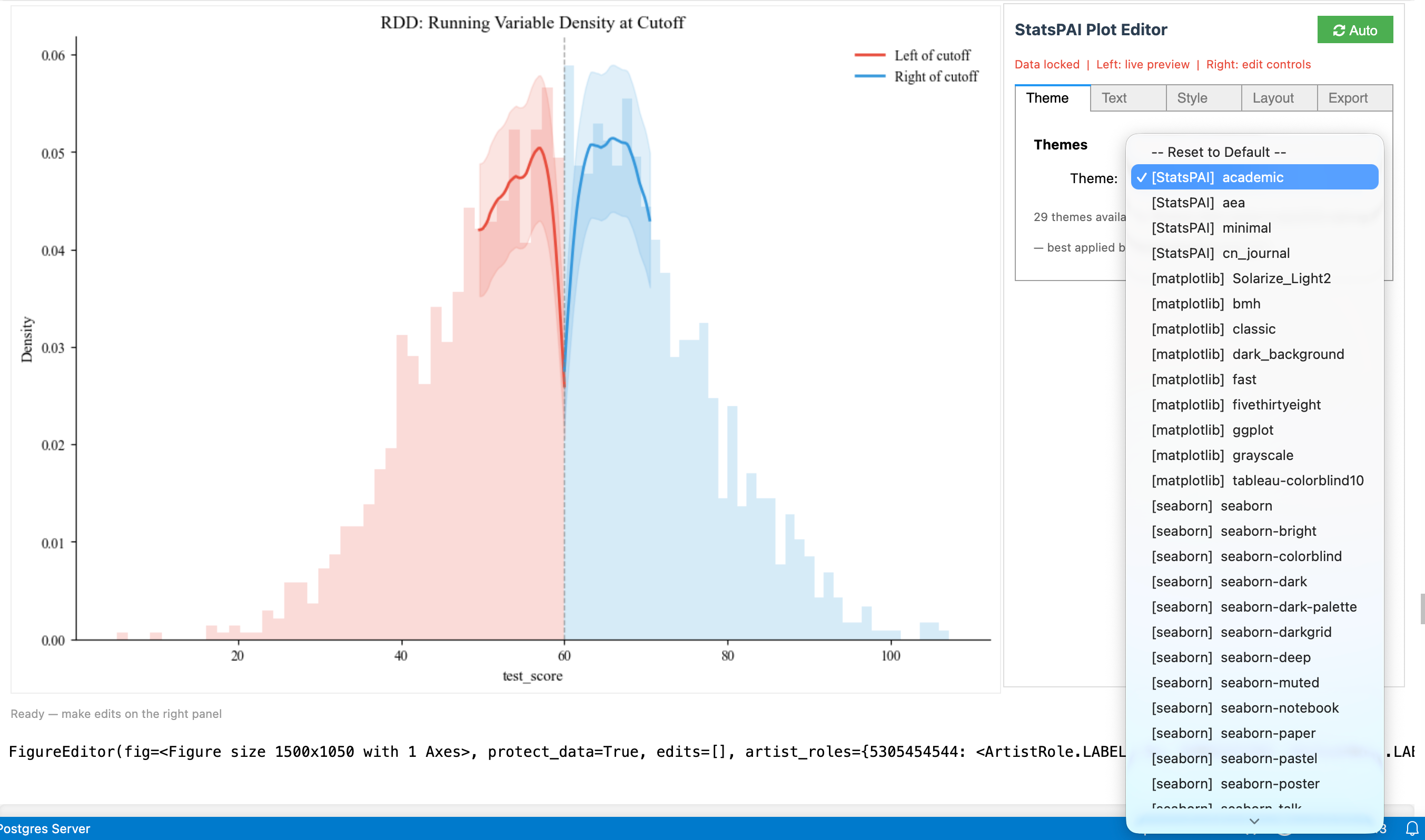
interactive()	WYSIWYG plot editor with 29 themes & auto code generation	Jupyter ipywidgets

Every result object has:

result.summary()      # Formatted text summary
result.plot()         # Appropriate visualization
result.to_latex()     # LaTeX table
result.to_docx()      # Word document
result.cite()         # BibTeX citation for the method

Interactive Plot Editor — Python's Answer to Stata Graph Editor

Stata users know the Graph Editor: double-click a figure to enter a WYSIWYG editing interface — drag fonts, change colors, adjust layout. This has been a Stata-exclusive experience. In Python, matplotlib produces static images — changing a title font size means editing code and re-running.

sp.interactive(fig) turns any matplotlib figure into a live editing panel — figure preview on the left, property controls on the right, just like Stata's Graph Editor. But it does two things Stata can't:

1. 29 academic themes, one-click switching. From AER journal style to ggplot, FiveThirtyEight, dark presentation mode — select and see the result instantly. Stata's scheme requires regenerating the plot; here it's real-time.

2. Every edit auto-generates reproducible Python code. Adjust title size, change colors, add annotations in the GUI — the editor records each operation as standard matplotlib code (ax.set_title(...), ax.spines[...].set_visible(...)). Copy with one click, paste into your script, and it reproduces exactly. Stata's Graph Editor cannot export edits to do-file commands.

Five tabs cover all editing needs: Theme (29 themes) · Text (titles, labels, fonts) · Style (line colors, widths, markers) · Layout (spines, grid, figure size, legend, axis limits) · Export (save, undo/redo, reset).

Auto/Manual rendering modes: Auto refreshes the preview on every change; Manual batches edits for a single Apply — useful for large figures or slow machines.

import statspai as sp

result = sp.did(df, y='wage', treat='policy', time='year')
fig, ax = result.plot()
editor = sp.interactive(fig)   # opens the editor

# After editing in the GUI:
editor.copy_code()             # prints reproducible Python code

Utilities

Function	Description	Stata equivalent
label_var(), label_vars()	Variable labeling	label var
describe()	Data description	describe
pwcorr()	Pairwise correlation with significance stars	pwcorr, star(.05)
winsor()	Winsorization	winsor2
read_data()	Multi-format data reader	use / import

---

Installation

pip install statspai

With optional dependencies:

pip install statspai[plotting]    # matplotlib, seaborn
pip install statspai[fixest]      # pyfixest for high-dimensional FE

Requirements: Python >= 3.9

Core dependencies: NumPy, SciPy, Pandas, statsmodels, scikit-learn, linearmodels, patsy, openpyxl, python-docx

---

Quick Example

import statspai as sp

# --- Estimation ---
r1 = sp.regress("wage ~ education + experience", data=df, robust='hc1')
r2 = sp.ivreg("wage ~ (education ~ parent_edu) + experience", data=df)
r3 = sp.did(df, y='wage', treat='policy', time='year', id='worker')
r4 = sp.rdrobust(df, y='score', x='running_var', c=0)
r5 = sp.dml(df, y='wage', treat='training', covariates=['age', 'edu', 'exp'])
r6 = sp.causal_forest("y ~ treatment | x1 + x2 + x3", data=df)

# --- Post-estimation ---
sp.margins(r1, data=df)              # Marginal effects
sp.test(r1, "education = experience") # Wald test
sp.oster_bounds(df, y='wage', treat='education', controls=['experience'])

# --- Tables (to Word / Excel / LaTeX) ---
sp.modelsummary(r1, r2, output='table2.docx')
sp.outreg2(r1, r2, r3, filename='results.xlsx')
sp.sumstats(df, vars=['wage', 'education', 'age'], output='table1.docx')

# --- Robustness (unique to StatsPAI) ---
sp.spec_curve(df, y='wage', x='education',
              controls=[[], ['experience'], ['experience', 'female']],
              se_types=['nonrobust', 'hc1']).plot()

sp.robustness_report(df, formula="wage ~ education + experience",
                     x='education', extra_controls=['female'],
                     winsor_levels=[0.01, 0.05]).plot()

sp.subgroup_analysis(df, formula="wage ~ education + experience",
                     x='education',
                     by={'Gender': 'female', 'Region': 'region'}).plot()

---

StatsPAI vs Stata vs R: Honest Comparison

Where StatsPAI wins

Advantage	Detail
Unified API	One package, one import, consistent .summary() / .plot() / .to_latex() across all methods. Stata requires paid add-ons; R requires 20+ packages with different interfaces.
Modern ML causal methods	DML, Causal Forest, Meta-Learners (S/T/X/R/DR), TMLE, DeepIV, TARNet/CFRNet/DragonNet, Policy Trees — all in one place. Stata has almost none of these. R has them scattered across incompatible packages.
Robustness automation	spec_curve(), robustness_report(), subgroup_analysis() — no manual re-running. Neither Stata nor R offers this out-of-the-box.
Free & open source	MIT license, $0. Stata costs $695–$1,595/year.
Python ecosystem	Integrates naturally with pandas, scikit-learn, PyTorch, Jupyter, cloud pipelines.
Auto-citations	Every causal method has .cite() returning the correct BibTeX. Neither Stata nor R does this.
Interactive Plot Editor	sp.interactive() — Stata Graph Editor-style GUI in Jupyter with 29 themes and auto-generated reproducible code. Stata's Graph Editor can't export edits to do-file; R has no equivalent.

Where Stata still wins

Advantage	Detail
Battle-tested at scale	40+ years of production use in economics. Edge cases are well-handled.
Speed on very large datasets	Stata's compiled C backend is faster for simple OLS/FE on datasets with millions of rows.
Survey data & complex designs	svy: prefix, stratification, clustering — Stata's survey support is unmatched.
Mature documentation	Every command has a PDF manual with worked examples. Community is massive.
Journal acceptance	Referees in some fields trust Stata output by default.

Where R still wins

Advantage	Detail
Cutting-edge methods	New econometric methods (e.g., fixest, did2s, HonestDiD) often appear in R first.
ggplot2 visualization	R's grammar of graphics is more flexible than matplotlib for complex figures.
modelsummary	R's modelsummary is the gold standard for regression tables — StatsPAI's is close but not yet identical.
CRAN quality control	R packages go through peer review. Python packages vary in quality.
Spatial econometrics	spdep, spatialreg — As of v0.8.0, StatsPAI matches R's 5-package spatial stack (spdep + spatialreg + sphet + splm + GWmodel) in a single unified API, with numerical parity to PySAL spreg at rtol<1e-7 on the Columbus benchmark.

---

API at a Glance

450+ public functions/classes

Regression:     regress, ivreg, glm, logit, probit, mlogit, ologit, poisson, nbreg, ppmlhdfe,
                tobit, heckman, qreg, truncreg, fracreg, betareg, sureg, three_sls, gmm
IV Advanced:    liml, jive, lasso_iv
Panel:          panel, panel_logit, panel_probit, panel_fgls, interactive_fe, xtabond, mixed
DID:            did, callaway_santanna, sun_abraham, bacon_decomposition, honest_did,
                continuous_did, did_multiplegt, did_imputation, stacked_did
RD:             rdrobust, rdplot, rddensity, rdmc, rdms, rkd
Matching:       match, ebalance, ipw, aipw
Synth:          synth, sdid, gsynth, augsynth, staggered_synth, conformal_synth
ML Causal:      dml, causal_forest, deepiv, metalearner, tmle
Neural:         tarnet, cfrnet, dragonnet
Spatial:        sar, sem, sdm, slx, sac, sar_gmm, sem_gmm, sarar_gmm,          ← NEW v0.8
                moran, geary, getis_ord_g, join_counts, lm_tests, impacts,
                gwr, mgwr, gwr_bandwidth, spatial_panel,
                queen_weights, rook_weights, knn_weights, distance_band, kernel_weights
Discovery:      notears, pc_algorithm, lingam, ges                              ← NEW v0.8
Policy:         policy_tree, policy_value
Survival:       cox, kaplan_meier, survreg, logrank_test, cox_frailty, aft      ← NEW v0.8
Time Series:    var, granger_causality, irf, structural_break, johansen,
                local_projections, garch, arima, bvar                           ← NEW v0.8
Nonparametric:  lpoly, kdensity
Experimental:   randomize, balance_check, attrition_test, optimal_design
Matching:       match, ebalance, optimal_match, cardinality_match               ← NEW v0.8
Decomposition:  oaxaca, gelbach, rifreg, rif_decomposition                      ← NEW v0.8
Imputation:     mice, mi_estimate
Frontier:       frontier (stochastic frontier analysis)
Structural:     blp (BLP demand estimation)
Survey:         svydesign, svymean, svytotal, svyglm, rake, linear_calibration  ← NEW v0.8
MR:             mendelian_randomization, mr_ivw, mr_egger, mr_median
Mediation:      mediate, mediate_sensitivity                                    ← NEW v0.8
RD:             rdrobust, rdplot, rddensity, rdmc, rdms, rdpower, rdsampsi      ← NEW v0.8
Smart Workflow: recommend, compare_estimators, assumption_audit,
                sensitivity_dashboard, pub_ready, replicate
Output:         modelsummary, outreg2, sumstats, balance_table, tab, coefplot, binscatter
Plot Editor:    interactive (WYSIWYG editor), set_theme (29 academic themes)

---

Release Notes

v0.9.3 (2026-04-19) — Stochastic Frontier + Multilevel + GLMM + Econometric Trinity

24 commits since 0.9.2 (includes the GLMM hardening pillar originally tagged as 0.9.4, folded into 0.9.3 before tag). See CHANGELOG for full detail.

⚠️ Critical correctness fix in sp.frontier. A latent Jondrow-posterior sign error in all prior versions (≤ 0.9.2) produced systematically biased efficiency scores; the dist='exponential' path additionally returned NaN for unit efficiency. Re-run any prior frontier analyses.

1. Stochastic Frontier — full Stata/R parity and beyond. sp.frontier + sp.xtfrontier rewritten (~2,700 LOC).

• Cross-sectional: heteroskedastic inefficiency usigma=[...] (Caudill-Ford-Gropper 1995), heteroskedastic noise vsigma=[...] (Wang 2002), inefficiency determinants emean=[...] (Kumbhakar-Ghosh-McGuckin 1991); Battese-Coelli (1988) E[exp(-u)|ε] alongside JLMS; LR mixed-χ̄² test (Kodde-Palm 1986); parametric-bootstrap unit-efficiency CIs.
• Panel: Pitt-Lee (1981) time-invariant; Battese-Coelli (1992) time-decay; Battese-Coelli (1995) full-flexibility; Greene (2005) TFE/TRE; Dhaene-Jochmans (2015) split-panel jackknife bias correction via xtfrontier(..., model='tfe', bias_correct=True).
• New advanced frontiers: sp.zisf — Zero-Inefficiency SFA mixture (Kumbhakar-Parmeter-Tsionas 2013); sp.lcsf — 2-class Latent-Class SFA (Orea-Kumbhakar 2004 / Greene 2005).
• Productivity: sp.malmquist — Färe-Grosskopf-Lindgren-Roos (1994) Malmquist TFP index with M = EC × TC decomposition; sp.translog_design — Cobb-Douglas → Translog design-matrix helper.
• Inference + post-estimation: vce='opg' / 'robust' / 'cluster' / 'bootstrap' with Monte-Carlo coverage check; conditional predict(), returns-to-scale, usigma / emean marginal effects, metafrontier.

2. Multilevel / Mixed-Effects — sp.multilevel rewritten. From a 400-LOC two-level single file to a ~2,700-LOC sub-package with lme4/Stata mixed parity. sp.mixed now defaults to unstructured random-effect covariance, supports three-level nested models (group=['school','class']), BLUP posterior SEs, Nakagawa-Schielzeth R², caterpillar plots. New top-level: sp.melogit / sp.mepoisson / sp.meglm (Laplace GLMMs), sp.icc (delta-method CI), sp.lrtest (Self-Liang χ̄² boundary correction). Verified against statsmodels.MixedLM to 4 decimal places.

3. GLMM hardening — AGHQ + Gamma / NegBin / Ordinal. Closes the three GLMM gaps flagged in the multilevel self-audit. Adaptive Gauss-Hermite quadrature via new nAGQ argument: nAGQ=1 reduces exactly to Laplace (verified 1e-10); nAGQ>1 matches Stata intpoints(7) / R lme4::glmer(nAGQ=7) accuracy on small clusters with binary or other non-Gaussian outcomes. Wired into all five families (Gaussian / Binomial / Poisson / Gamma / NegBin) plus meologit. New families: sp.megamma (Gamma GLMM, log link, ML-estimated dispersion log φ, Fisher-scoring IRLS), sp.menbreg (NB-2 Var = μ + αμ², reduces to Poisson as α → 0), sp.meologit (random-effects ordinal logit with K−1 reparameterised thresholds κ_1, log(κ_2−κ_1), … for unconditional ordering). Cross-family AIC comparability: Poisson and Binomial log-likelihoods now include full normalisation constants (-log(y!) / log-binomial-coefficient) so mepoisson vs menbreg AIC comparisons are unbiased.

4. Econometric Trinity — three new P0 pillars (~1,170 LOC).

• sp.dml(model='pliv', instrument=...) — Partially Linear IV (Chernozhukov et al. 2018, §4.2) with Neyman-orthogonal score and cross-fitted g/m/r nuisances; influence-function SEs.
• sp.mixlogit — Random-coefficient MNL via simulated ML with Halton draws. Normal / log-normal / triangular mixing; diagonal or Cholesky covariance; panel repeated-choice; OPG-sandwich SEs. Python's first feature-complete implementation.
• sp.ivqreg — Chernozhukov-Hansen IV quantile regression via inverse-QR profile. Grid + Brent (scalar endogenous); BFGS on b̂(α) (multi-dim); pairs-bootstrap SEs.

5. Smart workflow — posterior verification. sp.verify / sp.verify_benchmark — aggregates bootstrap stability + placebo pass rate + subsample agreement into a verify_score ∈ [0, 100] for any sp.recommend() output. Opt-in via recommend(verify=True); zero overhead when off.

Quality bar. Multilevel passed oracle + code-reviewer audit (4 BLOCKER + 5 HIGH fixed); econ-trinity passed self-audit (4 BLOCKER + 7 HIGH fixed); frontier self-audit fixed Mills-tail, TVD-loop, cost-panel, summary-dump issues. GLMM hardening added 18 new tests (TestAGHQ × 7, TestMEGamma × 3, TestMENegBin × 3, TestMEOLogit × 5) on top of the 35 prior multilevel tests. Test count: 93/93 frontier, 53/53 multilevel (incl. GLMM), 18/18 smart, 10/10 econ-trinity pass.

Meta. Author attribution corrected from "Bryce Wang" to "Biaoyue Wang" in pyproject.toml, __author__, English/Chinese READMEs, docs/index.md, and mkdocs.yml (JOSS paper.md was already correct).

v0.9.2 (2026-04-16) — Decomposition Analysis Mega-Release

Release focus: statspai.decomposition. 18 first-class decomposition methods across 13 modules (~6,200 LOC, 54 tests) — Python's first (and most complete) implementation of the full decomposition toolkit spanning mean, distributional, inequality, demographic, and causal decomposition. Occupies the previously empty Python high-ground where only one unmaintained 2018-vintage PyPI package existed.

18 methods (30 aliases) under sp.decompose():

• Mean — oaxaca (Blinder-Oaxaca threefold with 5 reference coefficients: Neumark 1988, Cotton 1988, Reimers 1983, group A, group B), gelbach (Gelbach 2016 sequential OVB), fairlie (nonlinear logit/probit), bauer_sinning / yun_nonlinear (detailed nonlinear)
• Distributional — rifreg / rif_decomposition (FFL 2009), ffl_decompose (FFL 2018 two-step), dfl_decompose (DiNardo-Fortin-Lemieux 1996 reweighting), machado_mata (MM 2005), melly_decompose (Melly 2005), cfm_decompose (Chernozhukov-Fernández-Val-Melly 2013)
• Inequality — subgroup_decompose (Theil T/L, GE(α), Dagum Gini, Atkinson, CV²), shapley_inequality (Shorrocks 2013), source_decompose (Lerman-Yitzhaki 1985)
• Demographic — kitagawa_decompose (1955), das_gupta (1993 multi-factor symmetric)
• Causal — gap_closing (Lundberg 2021 regression/IPW/AIPW), mediation_decompose (VanderWeele 2014 NDE/NIE), disparity_decompose (Jackson-VanderWeele 2018)

Quality bar:

• Closed-form influence functions for Theil T / Theil L / Atkinson (no O(n²) numerical fallback)
• Weighted O(n log n) Dagum Gini via sorted-ECDF pairwise-MAD identity
• Cross-method consistency tests (test_dfl_ffl_mean_agree, test_mm_melly_cfm_aligned_reference, test_dfl_mm_reference_convention_opposite)
• Numerical identity checks: FFL four-part sum, weighted Gini RIF E_w[RIF] = G
• Logit non-convergence surfaces as RuntimeWarning; bootstrap failure rate >5% warns
• 54 decomposition tests + core refactor consolidation: decomposition/_common.py hosts influence_function(y, stat, tau, w) — the canonical 9-statistic RIF kernel (rif.rif_values public API expands from 3 to 9 statistics)

Unified entry point:

import statspai as sp
result = sp.decompose(method='ffl', data=df, y='log_wage',
                      group='female', x=['education', 'experience'],
                      stat='quantile', tau=0.5)
result.summary(); result.plot(); result.to_latex()

v0.9.1 (2026-04-16) — Regression Discontinuity Mega-Upgrade

Release focus: statspai.rd. 18+ RD estimators, diagnostics, and inference methods across 14 modules (~10,300 LOC) — the most feature-complete RD package in Python, R, or Stata. Full machinery behind CCT, Cattaneo-Jansson-Ma density tests, Armstrong-Kolesar honest CIs, Cattaneo-Titiunik-Vazquez-Bare local randomization, Cattaneo-Titiunik-Yu boundary (2D) RD, and Angrist-Rokkanen external validity — all under sp.*.

Core estimation:

• rdrobust — sharp / fuzzy / kink RD with bias-corrected robust inference (CCT 2014); covariate-adjusted local polynomial (CCFT 2019)
• rd2d — boundary discontinuity / 2D RD (Cattaneo, Titiunik & Yu 2025)
• rkd — Regression Kink Design (Card, Lee, Pei & Weber 2015)
• rdit — Regression Discontinuity in Time (Hausman & Rapson 2018)
• rdmc, rdms — multi-cutoff and multi-score RD

Bandwidth selection: rdbwselect with mserd, msetwo, cerrd, cercomb1, cercomb2 (Imbens-Kalyanaraman 2012; CCF 2020).

Inference:

• rd_honest — honest CIs with worst-case bias bound (Armstrong-Kolesar 2018, 2020)
• rdrandinf, rdwinselect, rdsensitivity — local randomization inference (Cattaneo-Frandsen-Titiunik 2015)
• rdrbounds — Rosenbaum sensitivity bounds for hidden selection

Heterogeneous treatment effects: rdhte (CATE via fully interacted local linear), rdbwhte, rd_forest, rd_boost, rd_lasso.

External validity & extrapolation: rd_extrapolate (Angrist-Rokkanen 2015), rd_multi_extrapolate (CKTV 2024).

Diagnostics & one-click dashboard: rdsummary (rdrobust + density test + bandwidth sensitivity + placebo cutoffs + covariate balance), rdplot (IMSE-optimal binning), rddensity (CJM 2020), rdbalance, rdplacebo.

Power analysis: rdpower, rdsampsi.

Refactor — rd/_core.py: 5-sprint refactor consolidated shared low-level primitives duplicated across 9 RD files into one 191-line canonical private module (_kernel_fn, _kernel_constants, _local_poly_wls, _sandwich_variance). 253 lines of duplicated math → 191 lines of canonical implementation. 97 RD tests pass with zero regression.

Also in 0.9.1:

• synth/_core.py — simplex weight solver consolidated from 6 duplicate implementations; analytic Jacobian now available to all six callers (~3-5× speedup)
• Bug fixes: density test CJM (2020) implementation + DGP helpers + validation tests; 3 critical + 3 high-priority bugs from comprehensive RD code review; _ols_fit singular matrix fallback

v0.9.0 (2026-04-16) — Synthetic Control Mega-Expansion

Release focus: statspai.synth. 20 SCM methods + 6 inference strategies + full research workflow (compare / power / sensitivity / one-click reports), all behind the unified sp.synth(method=...) dispatcher. No competing package in Python, R, or Stata offers this breadth.

Seven new SCM estimators:

Method	Reference
bayesian_synth	Dirichlet-prior MCMC with full posterior credible intervals (Vives & Martinez 2024)
bsts_synth / causal_impact	Bayesian Structural Time Series via Kalman filter/smoother (Brodersen et al. 2015)
penalized_synth (penscm)	Pairwise discrepancy penalty (Abadie & L'Hour 2021, JASA)
fdid	Forward DID with optimal donor subset selection (Li 2024)
cluster_synth	K-means / spectral / hierarchical donor clustering (Rho 2024)
sparse_synth	L1 / constrained-LASSO / joint V+W (Amjad, Shah & Shen 2018, JMLR)
kernel_synth + kernel_ridge_synth	RKHS / MMD-based nonlinear matching

Previous methods — classic, penalized, demeaned, unconstrained, augmented (ASCM), SDID, gsynth, staggered, MC, discos, multi-outcome, scpi — remain with bug fixes.

Research workflow:

• synth_compare(df, ...) — run every method at once, tabular + graphical comparison
• synth_recommend(df, ...) — auto-select best estimator by pre-fit + robustness
• synth_report(result, format='markdown'|'latex'|'text') — one-click publication-ready report
• synth_power(df, effect_sizes=[...]) — first power-analysis tool for SCM designs
• synth_mde(df, target_power=0.8) — minimum detectable effect
• synth_sensitivity(result) — LOO + time placebos + donor sensitivity + RMSPE filtering
• Canonical datasets: california_tobacco(), german_reunification(), basque_terrorism()

Release-blocker fixes (5-parallel-agent code review — correctness / numerics / API / perf / docs):

• ASCM correction formula — augsynth now follows Ben-Michael, Feller & Rothstein (2021) Eq. 3 per-period ridge bias (Y1_pre − Y0'γ) @ β(T0, T1), replacing the scalar mean-residual placeholder; _ridge_fit RHS bug also fixed
• Bayesian likelihood scale — covariate rows z-scored to pooled pre-outcome SD before concatenation
• Bayesian MCMC Jacobian — missing log(σ′/σ) correction for log-normal random-walk proposal on σ added to MH acceptance ratio
• BSTS Kalman filter — innovation variance floored at 1e-12; RTS smoother inv → solve + pinv fallback on near-singular predicted covariance
• gsynth factor estimation — four np.linalg.inv → np.linalg.lstsq (robust to rank-deficient F'F / L'L)
• Dispatcher **kwargs leakage fixed for augsynth and kernel_ridge placebo forwarding
• Cross-method API consistency — sdid() accepts canonical outcome / treated_unit / treatment_time (legacy aliases retained)

Tests & validation: 144 synth tests passing (new: 12-method cross-method consistency benchmark). Full suite: 1481 passed, 4 skipped, 0 failed. New guide: docs/guides/synth.md with a 20-method decision table.

v0.8.0 (2026-04-16) — Spatial Econometrics Full-Stack + 10-Domain Breadth Upgrade

60+ new functions, 450+ total API, 1,230+ tests passing. Largest release in StatsPAI history.

Spatial Econometrics (NEW — 38 API symbols, 3,178 LOC, 69 tests):

• Weights: W (sparse CSR), queen_weights, rook_weights, knn_weights, distance_band, kernel_weights, block_weights
• ESDA: moran (global + local LISA), geary, getis_ord_g, getis_ord_local, join_counts, moran_plot, lisa_cluster_map
• ML Regression: sar, sem, sdm, slx, sac (SARAR) — sparse-aware, scales to N=100K
• GMM Regression: sar_gmm, sem_gmm, sarar_gmm (Kelejian-Prucha 1998/1999, het-robust)
• Diagnostics: lm_tests (Anselin 1988 — LM-err/LM-lag/Robust-LM/SARMA), moran_residuals
• Effects: impacts (LeSage-Pace 2009 direct/indirect/total with simulated SE)
• GWR: gwr, mgwr (Multiscale GWR), gwr_bandwidth (AICc/CV golden-section)
• Spatial Panel: spatial_panel (SAR-FE / SEM-FE / SDM-FE, entity + twoways)
• Cross-validated: Columbus SAR/SEM rtol<1e-7 vs PySAL spreg; Georgia GWR bit-identical vs mgwr

Time Series (4 new estimators):

• local_projections — Jordà (2005) horizon-by-horizon IRF with Newey-West HAC
• garch — GARCH(p,q) volatility model, MLE, multi-step forecast
• arima — ARIMA/SARIMAX with auto (p,d,q) selection via AICc grid
• bvar — Bayesian VAR with Minnesota (Litterman) prior, closed-form posterior

Causal Discovery (2 new algorithms):

• lingam — DirectLiNGAM (Shimizu 2011), bit-identical match vs lingam package
• ges — Greedy Equivalence Search (Chickering 2002), BIC-based CPDAG learning

Matching (2 new methods):

• optimal_match — global 1:1 matching via Hungarian algorithm (min total Mahalanobis distance)
• cardinality_match — Zubizarreta (2014) LP-based matching with SMD balance constraints

Decomposition & Mediation:

• rifreg — RIF regression (Firpo-Fortin-Lemieux 2009), unconditional quantile partial effects
• rif_decomposition — RIF Oaxaca-Blinder for distributional statistics
• mediate_sensitivity — Imai-Keele-Yamamoto (2010) ρ-sensitivity analysis

RD & Design:

• rdpower, rdsampsi — power calculations for RD designs (Cattaneo et al. 2019)

Survey:

• rake — iterative proportional fitting (Deming-Stephan) for survey calibration
• linear_calibration — Deville-Särndal (1992) chi-squared distance calibration

Survival (2 new models):

• cox_frailty — Cox proportional hazards with shared gamma frailty
• aft — Accelerated Failure Time (exponential/Weibull/lognormal/loglogistic)

ML-Causal (GRF extensions):

• CausalForest.variable_importance() — permutation-based feature importance for CATE
• CausalForest.best_linear_projection() — BLP heterogeneity test (Chernozhukov et al. 2020)
• CausalForest.ate(), .att() — convenience accessors
• Bugfix: honest leaf values now correctly vary per-leaf (was overwriting all leaves)

Infrastructure:

• OLS/IV predict(data, what='confidence'|'prediction') — out-of-sample with intervals
• Pre-release code review: 3 critical + 2 high-priority bugs fixed before release

v0.6.0 (2026-04-05) — Complete Econometrics Toolkit + Smart Workflow Engine

30 new modules, 390+ public API, 860+ tests passing, 83K+ lines of code.

New Regression & GLM:

• glm() (6 families × 8 links), logit(), probit(), cloglog(), mlogit(), ologit(), oprobit(), clogit()
• poisson(), nbreg(), ppmlhdfe() (gravity model), zip_model(), zinb(), hurdle()
• truncreg(), fracreg(), betareg(), biprobit(), etregress()
• liml(), jive(), lasso_iv() (advanced IV), sureg(), three_sls(), gmm() (general GMM)

New Panel & Multilevel:

• panel_logit(), panel_probit() (FE/RE/CRE), panel_fgls(), interactive_fe() (Bai 2009)
• panel_unitroot() (IPS/LLC/Fisher/Hadri), mixed() (multilevel/HLM)

New Survival: cox(), kaplan_meier(), survreg(), logrank_test()

New Time Series: var(), granger_causality(), irf(), structural_break(), cusum_test(), engle_granger(), johansen()

New Causal: continuous_did(), rdmc(), rdms() (geographic RD), distributional_te(), mendelian_randomization()

New Design & Data: randomize(), balance_check(), attrition_test(), optimal_design(), mice(), mi_estimate()

New Structural: blp() (BLP demand estimation), frontier() (stochastic frontier)

Smart Workflow Engine (unique to StatsPAI):

• recommend() — data + question → estimator recommendation + workflow
• compare_estimators() — multi-method comparison with agreement diagnostics
• assumption_audit() — one-call assumption testing with remedies
• sensitivity_dashboard() — multi-dimensional sensitivity analysis
• pub_ready() — journal-specific publication readiness checklist
• replicate() — built-in famous datasets with replication guides

Interactive Plot Editor: Font presets redesigned to show actual font names; separate font and size presets for independent per-element control.

v0.6.2 (2026-04-12) — Weights, Prediction & Validation

• OLS predict(): Out-of-sample prediction via result.predict(newdata=)
• balance_panel(): Keep only units observed in every period
• DID/DDD/Event Study weights: weights= parameter for population-weighted estimation
• Matching ps_poly=: Polynomial propensity score models (Cunningham 2021, Ch. 5)
• Synth RMSPE plot: synthplot(result, type='rmspe') histogram (Abadie et al. 2010)
• Graddy (2006) replication: Fulton Fish Market IV example in sp.replicate()
• Numerical validation: Cross-validated against Stata/R reference values

v0.6.1 (2026-04-07) — Interactive Editor Fixes & Improvements

• Theme switching fix: Themes now fully reset rcParams before applying, so switching between themes (e.g. ggplot → academic) correctly updates all visual properties
• Apply button fix: Fixed being clipped on the Layout tab; now pinned to panel bottom
• Error visibility: Widget callback errors now surface in the status bar instead of being silently swallowed
• Auto mode: Always refreshes preview when toggled for immediate feedback
• Theme tab: Moved to first position; color pickers show confirmation feedback
• Code generation: Auto-generate reproducible code with text selection support

v0.5.1 (2026-04-04) — Interactive Plot Editor & Agent Enhancements

v0.4.0 (2026-04-05) — Module Architecture Overhaul

Major refactoring and expansion of core modules (+5,800 lines of new code):

• DID: Added Triple Differences (ddd()), one-call did_analysis() workflow (auto design detection → Bacon decomposition → estimation → event study → sensitivity), and 8 publication-ready plot functions (parallel_trends_plot, bacon_plot, group_time_plot, enhanced_event_study_plot, treatment_rollout_plot, sensitivity_plot, cohort_event_study_plot)
• Synthetic Control: Modular rewrite — demeaned_synth(), robust_synth() (penalized SCM), gsynth() (Generalized SCM with interactive fixed effects), staggered_synth() (multi-unit staggered adoption), conformal_synth() (distribution-free inference), and comprehensive synth_plot() / synth_weight_plot() / synth_gap_plot()
• Panel: Major expansion of panel() — Hausman test, Breusch-Pagan LM, Pesaran CD, Wooldridge autocorrelation, panel unit root tests; added panel_summary_plot(), fe_plot(), re_comparison_plot()
• RD: New rd_diagnostics() suite — bandwidth sensitivity, placebo cutoffs, donut-hole robustness, covariate balance at cutoff, density test
• IV / 2SLS: Rewritten ivreg() with proper first-stage diagnostics (Cragg-Donald, Kleibergen-Paap), weak IV detection, Sargan-Hansen overidentification test, Anderson canonical correlation test, Stock-Yogo critical values
• Matching: Enhanced match() — added CEM (Coarsened Exact Matching), optimal matching, genetic matching; improved balance diagnostics with Love plot and standardized mean difference
• DAG: Expanded dag() with 15+ built-in example DAGs (dag_example()), dag_simulate() for data generation from causal graphs, backdoor/frontdoor criterion identification
• Causal Impact: Enhanced Bayesian structural time-series with automatic model selection and improved inference
• AI Agent Registry: Expanded list_functions(), describe_function(), function_schema(), search_functions() for LLM/agent tool-use integration
• CausalResult: Added .to_json(), .to_dict(), enhanced .summary() formatting

v0.3.1 (2025-12-20)

• Fix PyPI badge displaying stale version

v0.3.0 (2025-12-20) — ML & Advanced Causal Methods

• Meta-Learners: S/T/X/R/DR-Learner for CATE estimation with compare_metalearners() and CATE diagnostics (gate_test, blp_test)
• Neural Causal Models: TARNet, CFRNet, DragonNet for deep CATE estimation
• Causal Discovery: notears() (continuous DAG optimization), pc_algorithm() (constraint-based)
• TMLE: Targeted Maximum Likelihood Estimation with Super Learner
• Policy Learning: policy_tree() optimal treatment rules, policy_value() evaluation
• Conformal Causal: Distribution-free prediction intervals for ITE
• Bayesian Causal Forest: bcf() with separate prognostic/treatment functions
• Dose-Response: Continuous treatment GPS curves
• Bounds: Lee bounds (sample selection), Manski bounds (partial identification)
• Interference: spillover() direct + indirect effect decomposition
• DTR: g_estimation() multi-stage optimal treatment regimes
• Multi-Treatment: AIPW for multi-valued treatments
• Bunching: Kink/notch bunching estimator with elasticity
• Matrix Completion: mc_panel() nuclear-norm panel estimator
• Robustness: spec_curve(), robustness_report(), subgroup_analysis()
• New Regression: DeepIV, Heckman selection, quantile regression, Tobit, Arellano-Bond GMM
• New Diagnostics: E-value, Anderson-Rubin weak IV test, Sensemakr, RD density test
• Other: Entropy balancing, Sun-Abraham event study, Bacon decomposition, HonestDiD

v0.2.0 (2025-11-15) — Post-Estimation & Output

• Post-Estimation: margins(), marginsplot(), test(), lincom()
• Output Tables: modelsummary(), outreg2(), sumstats(), balance_table(), tab(), coefplot(), binscatter()
• Inference: wild_cluster_bootstrap(), aipw(), ri_test()
• New Modules: DML, Causal Forest, Matching (PSM/Mahalanobis), Synthetic Control (ADH + SDID), Panel (FE/RE/FD), Causal Impact, Mediation, Bartik IV
• Diagnostics: oster_bounds(), mccrary_test(), hausman_test(), het_test(), reset_test(), vif()
• Utilities: Variable labeling, describe(), pwcorr(), winsor(), read_data()

v0.1.0 (2025-10-01) — Initial Release

• Core regression: regress() OLS with robust/clustered/HAC standard errors
• Instrumental variables: ivreg() 2SLS
• Difference-in-Differences: did(), did_2x2(), callaway_santanna()
• Regression discontinuity: rdrobust()
• Unified CausalResult object with .summary(), .plot(), .to_latex(), .to_docx(), .cite()

---

About

StatsPAI Inc. is the research infrastructure company behind CoPaper.AI — the AI co-authoring platform for empirical research, born out of Stanford's REAP program.

CoPaper.AI — Upload your data, set your research question, and produce a fully reproducible academic paper with code, tables, and formatted output. Powered by StatsPAI under the hood. copaper.ai

Team:

• Biaoyue Wang — Founder. Economics, Finance, CS & AI. Stanford REAP.
• Dr. Scott Rozelle — Co-founder & Strategic Advisor. Stanford Senior Fellow, author of Invisible China.
• 

---

Contributing

git clone https://github.com/brycewang-stanford/statspai.git
cd statspai
pip install -e ".[dev,plotting,fixest]"
pytest

---

Citation

@software{wang2025statspai,
  title={StatsPAI: The Causal Inference & Econometrics Toolkit for Python},
  author={Wang, Biaoyue},
  year={2026},
  url={https://github.com/brycewang-stanford/statspai},
  version={1.5.0}
}

License

MIT License. See LICENSE.

---

GitHub · PyPI · User Guide · CoPaper.AI