📄 Theory 📄 my study notes whilst undertaking my stats class "Statistics required for AI & Machine learning"
This MD was styled and edited in StackEdit.io
- Introduction
- Descriptive Statistics 1
- Descriptive Statistics 2
- Probability
- Conditional Probability
- Discrete probability distribution
- Continuous probability distribution
- Statistical inference
- Hypothese test
- Ch-squared test
- ANOVA
- Simple regression
- Multiple regression
- Presentation of 6 distributions
- presentation Slides
Introduction
Source: https://www.selecthub.com/business-intelligence/statistical-software/
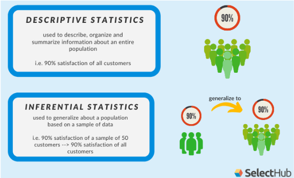
Descriptive Statistics Descriptive statistics involves describing, summarizing and organizing the data, so it can be easily understood Graphical display are often used along with the Quantitative measures to enable clarity of communication
- Used to describe, organise and summarise information about an entire data set
- So that it can be easily understood
- Graphical display are often used along with the Quantitative measures to clearly communication findings
- I.e 5% defect product production rate
- Used to generalise about a data set based on a sample of data
- I.e 5% defect product production rate of 30 projects —> 5% defect product production rate

Source: https://www.tes.com/teaching-resource/mean-median-mode-and-range-posters-12024923
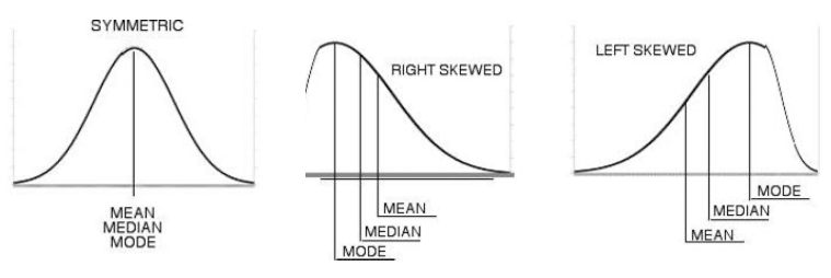
Mean, Median, and Mode (distribution curve)
Source: https://www.tes.com/teaching-resource/mean-median-mode-and-range-posters-12024923
Variance, and Standard Deviation

Source: https://byjus.com/maths/variance-and-standard-deviation/
Variance
- σ2 sigma squared is the symbol for variance
- mathematical terms frequently used in statistics and probability theory
- Variance refers to the spread of a data set around its mean value
- AKA the more clumped the data, the less variance there is in the values of the dataset. Where as a high variance will have numbers spread across the board.
- “If you pick a number, what are the chances its around the mean?”
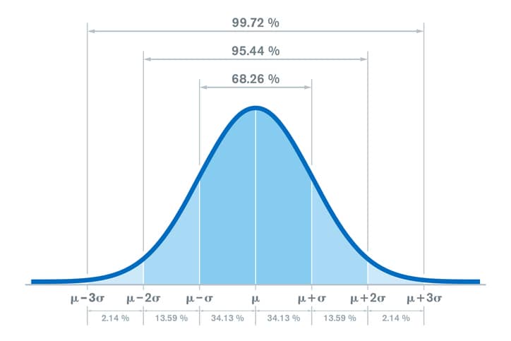
Standard Deviation
- Any data set that represents a Bell curve/normal distribution can be very useful. Because now Standard deviation applies to this dataset, we can extract cool information from it
- σ - greek sigma
- measures the spread of the data about the mean value (average)
- It is useful in comparing sets of data which may have the same mean but a different range
- For example,
- the mean of the following two is the same:
- 15, 15, 15, 14, 16 (avg 62) - 2, 7, 14, 22, 30. (avg 62) - However, the second is clearly more spread out.
- low standard deviation = the values are not spread out and clumped around the mean
- high standard deviation = the values are spread out and the curve is ‘flatter’
- How do the values deviate from the standard mean
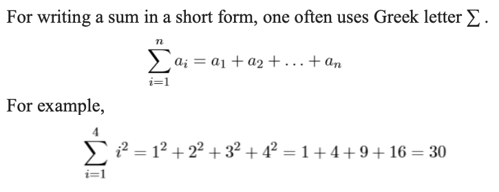
Sum Notation - ∑ [ˈsɪɡmə]
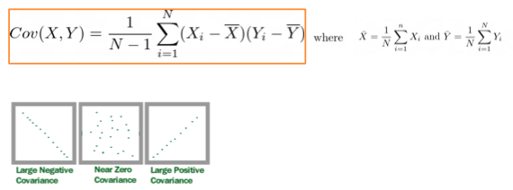
Covariance
- covariance is a measure of the relationship between two random variables.
- The metric evaluates how much – to what extent – the variables change together.
- Covariance values are not standardised
- E.G: COVID cases increase - available hospital beds decrease — Increase in daily exercise - decrease in weight
- Measures how 2 data sets Correlate
- 1 = as one grows, the other also grows as much
- -1 = as one grows, the other shrinks as much
- Covariance is when two variables vary with each other, whereas
- Correlation is when the change in one variable results in the change in another variable.
- https://www.mygreatlearning.com/blog/covariance-vs-correlation/
Source: https://www.tes.com/teaching-resource/mean-median-mode-and-range-posters-12024923
Correlation - Covariance is when two variables vary with each other, whereas - Correlation is when the change in one variable results in the change in another variable.
- IS covariance BUT not just linear direction but ALSO strength
- Based on covariance
- Covariance values are standardised

Source: https://www.datadeck.com/en/blog/2018/11/28/data-analytics-correlation-vs-causality/
Model
- Example: An ice cream company keeps track of how many ice creams get sold on different days(real world data).
- By comparing this to the weather on each day they can make a mathematical model of sales versus weather.
- They can then predict future sales based on the weather forecast, and decide how many ice creams they need to make ahead of time
Probability and Statics are polar opposites
- Probability creates models from real world data
- Statistics creates real world data from models

Source: https://daily.jstor.org/florence-nightingale-data-visualization-visionary/
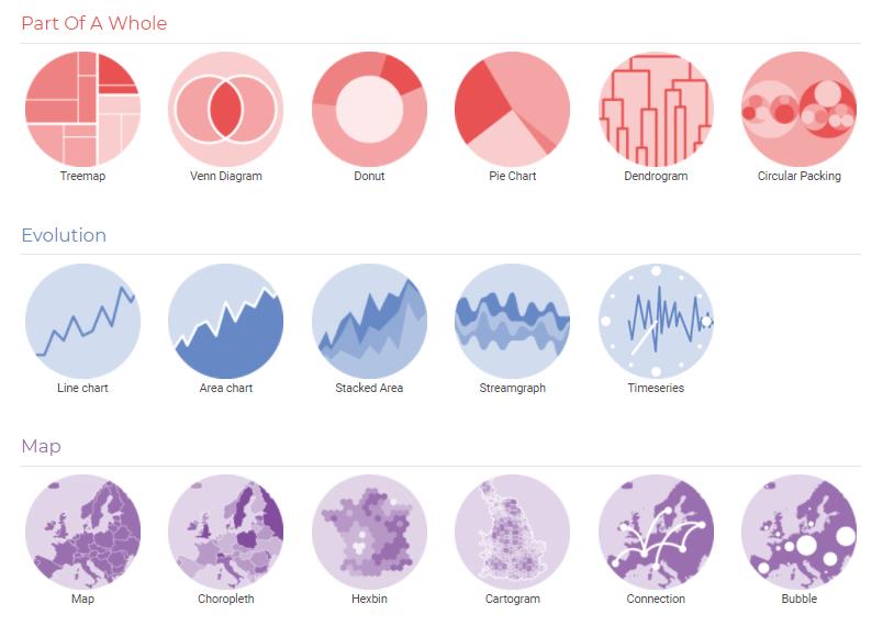
Data Visualisation
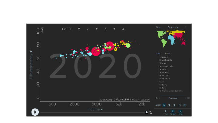
Source: https://www.gapminder.org/
Bar Chart (bar graph, or column chart)
A bar chart presents categorical data with rectangular bars with heights or lengths proportional to the values that they represent. A bar graph shows comparisons among discrete categories.

Source: https://en.wikipedia.org/wiki/Bar_chart
Line Chart (line plot, or curve chart)
A line chart displays information as a series of data points connected by straight line segments. A line chart is often used to visualize a trend in data over intervals of time – a time series.
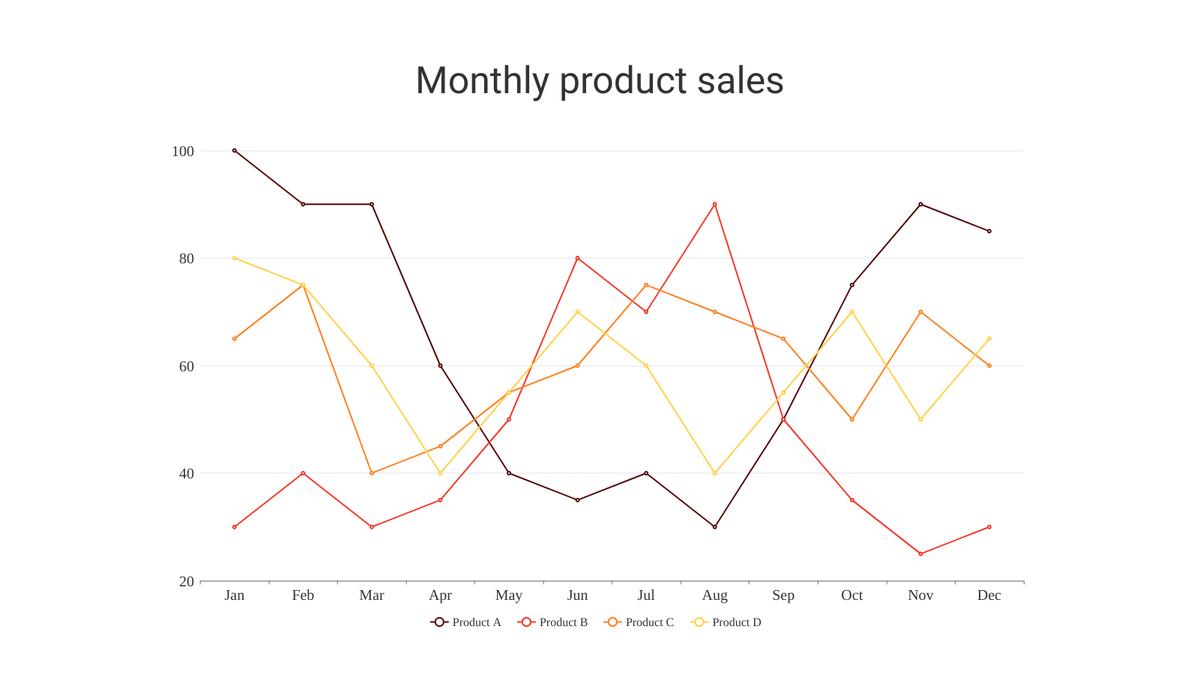
Source: https://en.wikipedia.org/wiki/Line_chart , https://online.visual-paradigm.com/charts/templates/line-charts/
Pie Chart (circle chart)
A pie chart is a circular statistical graphic, which is divided into slices to illustrate numerical proportion.
populations of English native speakers
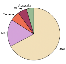
Source: https://en.wikipedia.org/wiki/Pie_chart
Radar chart (spider chart, web chart)
A radar chart displays multivariate data in the form of a two-dimensional chart to display multivariate observations. One application is quality control, i.e., analysis of strengths and weaknesses.
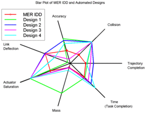
Source: https://en.wikipedia.org/wiki/Radar_chart
Histogram
A histogram is an approximate representation of the distribution of numerical data.
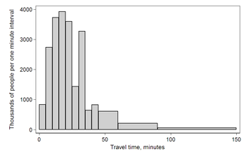
Source: https://en.wikipedia.org/wiki/Histogram
Scatter plot (scatter chart, scatter graph)
A scatter plot uses Cartesian coordinates to display values for typically two variables for a set of data, to identify the type of relationship (if any) between two quantitative variables
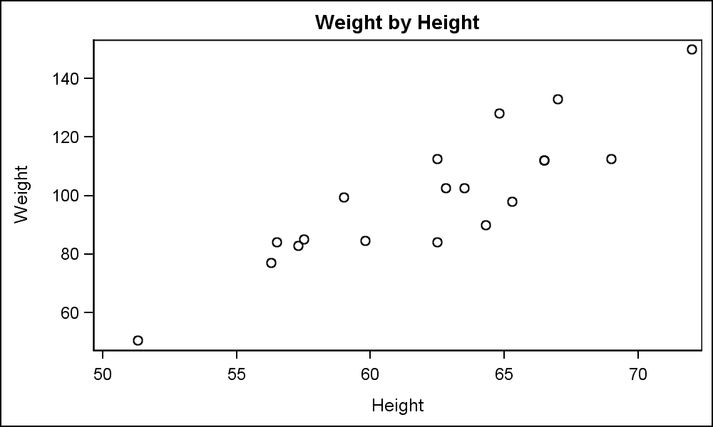
Source: https://en.wikipedia.org/wiki/Scatter_plot , https://blogs.sas.com/content/graphicallyspeaking/2016/10/04/getting-started-sgplot-part-1-scatter-plot/
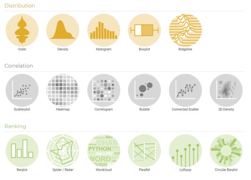
Charts with Python
- You can check the python code to plot various type of charts at “Python Graph Gallery”,
- https://www.python-graph-gallery.com/
Counting (Permutation & Combination)
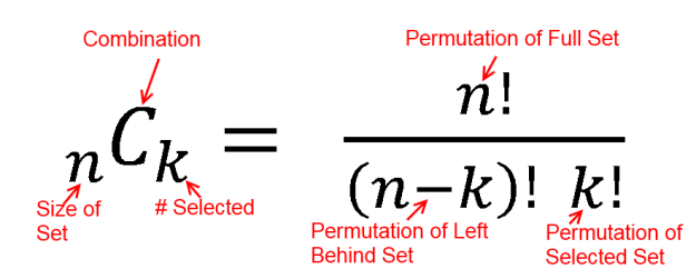
Combinations
- When the order of the data set does not matter, it is a combination
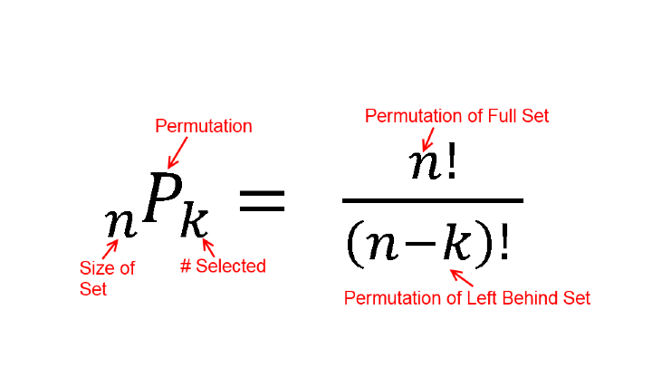
Permutation
- When the order of the data set does matter, it is a permutation
- A permutation is a ordered combination
- 2 types of permutation
- Repetition is allow - e.g a password 3333
- Repetition is not allowed - e.g if 3 people are running a race, they can not all be 1. It must be 1 2 and 3
- Repetition - Easy - n^r
- A lock has n dials from 1-10. That is n x n x n, or 10x10x10. Or 1000 possible combinations
- Or, more properly written n^r. N is the number of dials, r is the range (1 to 10)
- No repetition - okay - !n
- Example: what order could 16 pool balls be in?
- E.g 1: the idea is -> we pick ball x. Now there is 15 left. We pick ball y. Now there are 14 left
- 16 × 15 × 14 × 13 × ... = 20,922,789,888,000
- E.g 2: we only want the permutations of 3 pool balls
- 16 × 15 × 14 = 3,360
- In other words, there are 3,360 different ways that 3 pool balls could be arranged out of 16 balls.
- We write this as Factorial.
- 16 balls = !16 = 16 × 15 × ... = 20,922,789,888,000
- 3 balls = !16 / !13 = 16 × 15 x … / 13 × 14 x … = 3,360
Permutation
We have 5 participants for a competition, how many possible cases do we have for “who got which prize”?

We have 5 participants for a competition, how many possible cases do we have for “who got which prize”?
5 X4 X3

Source: http://www.fairlynerdy.com/permutations_and_combinations_simplified/ , 2020.10.04
Permutation with repetition
How many combinations in the pass-number for this lock?

Combination We have 5 participants for a competition, how many possible cases do we have if we are to choose 3 winners? 🏆🏆🏆 We have 5 participants for a competition, how many possible cases do we have if there’re “3 first place prizes”? ( 5 X 4 X 3 )/ ( 3 X 2X 1 )
How many combinations in the pass-number for this lock? 10 X 10 X 10 X 10
Source: http://www.fairlynerdy.com/permutations_and_combinations_simplified/ , 2020.10.04
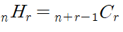
There are 3 types of fruits (apple, pear, orange), and you’re going to buy 5 fruits. How many combinations you can have?
oo/oo/o
Probability
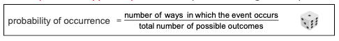
- Number of Desired outcome / number of total possible outcomes
- Number of times ill drink water a day / number of times a drink anything a day
Probability – the chance that an uncertain event will occur (always between 0 and 1)
Impossible Event – an event that has no chance of occurring (probability = 0)
Certain Event – an event that is sure to occur (probability = 1)
Source: https://learnzillion.com/lesson_plans/1413-the-addition-rule-for-the-probability-of-disjoint-events/

Source: https://www.wikihow.com/Understand-Probability
Probability of getting A+ ?
of favorable event: “Getting A+” = 1
of total events: “Getting A+”, “not Getting A+” = 2
Source: https://www.youtube.com/watch?v=eHJ40sSkYLE
What’s the probability of having breast cancer?
- 1% of women have breast cancer
- A woman got a mammogram detection of a breast cancer
- 80% of mammograms detect breast cancer when it is there
- 9.6% of mammograms detect breast cancer when it’s not there
- 1 around 80%, 2 over 50% 3 between 10% and 50% 4 less than 10%
Basic probability
- Probability – the chance that an uncertain event will occur (always between 0 and 1)
- Impossible Event – an event that has no chance of occurring (probability = 0)
- Certain Event – an event that is sure to occur (probability = 1)
Assessing probability
- A Priori (Classical approach) – based on prior knowledge of the process
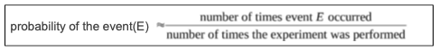
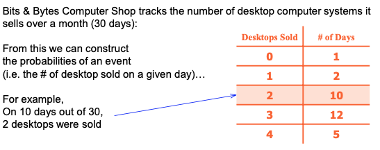
- Empirical probability (Relative frequency) – based on observation from experiment or historical events
- Subjective probability – based on a combination of an individual’s past experience, personal opinion, and analysis of a particular situation
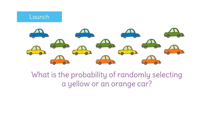
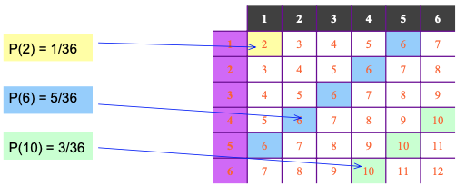
A Priori (Classical Approach)
-
Rolling two dice and probability of the total outcomes becomes {2, 3, ..., 12}
-
Empirical Probability (Relative Freq. Approach)
Subjective Probability
- “In the subjective approach we define probability as the degree of belief that we hold in the occurrence of an event”
- E.g. weather forecasting’s “P.O.P.”
- “Probability of Precipitation” (or P.O.P.) is defined in different ways by different forecasters, but basically it’s a subjective probability based on past observations combined with current weather conditions.
- POP 60% – based on current conditions, there is a 60% chance of rain (say).
Event
- Simple event
- An event described by a single characteristic o e.g. A day in January in 2020
- Joint event
- An event described by two or more characteristics
- e.g. A day in January that is also a Wednesday in 2020
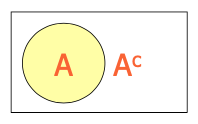
- Complement of an event A (denoted Ac)
- All events that are not part of event A
- e.g. All other days in 2020 that are not in January
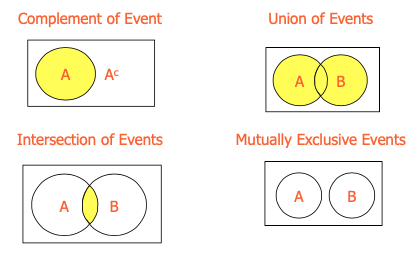
Organising and visualising events

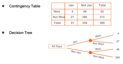
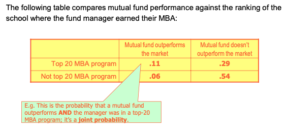
Joint, Marginal, Conditional Probability... We study methods to determine probabilities of events that result from combining other events in various ways. There are several types of combinations and relationships between events:
- Complement event
- Intersection of events
- Union of events
- Mutually exclusive events
- Dependent and independent events
Complement of an Event... The complement of event A is defined to be the event consisting of all sample points that are “not in A”. Complement of A is denoted by Ac The Venn diagram below illustrates the concept of a complement.
P(A)+P(Ac )=1
Intersection of Two Events...
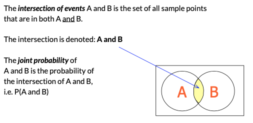
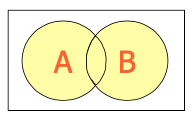
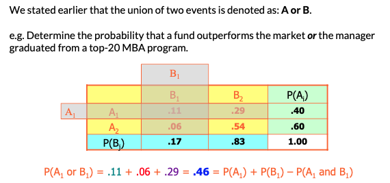
Union of Two Events...
The union of two events A and B, is the event containing all sample points that are in A or B or both:
Union of A and B is denoted: A or B
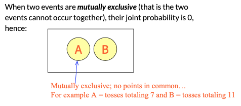
Mutually Exclusive Events...
Basic Relationships of Probability...
Example 6.1...
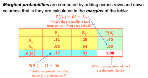
Marginal Probabilities...
Union...
Example 6.7... In a large city, two newspapers are published, the Sun and the Post.
- 22% of the city’s households have a subscription to the Sun
- 35% subscribe to the Post.
- A survey reveals that 6% of all households subscribe to both newspapers. What proportion of the city’s households subscribe to either newspaper?
- P(Sun or Post) = P(Sun) + P(Post) – P(Sun and Post) =.22+.35–.06=.51 “There is a 51% probability that a randomly selected household subscribes to one or the other or both papers” 6.44
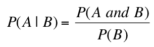
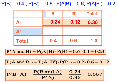
Conditional Probability... Conditional probability is used to determine the probability of one event given the occurrence of another related event. Conditional probabilities are written as P(A | B) and read as “the probability of A given B” and is calculated as:
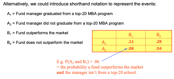
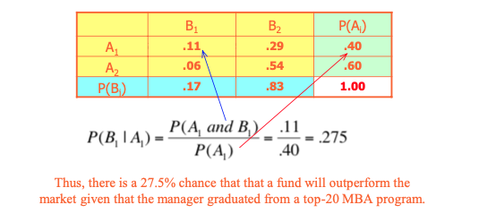
Example 6.2 What’s the probability that a fund will outperform the market given that the manager graduated from a top-20 MBA program? Recall: A1 = Fund manager graduated from a top-20 MBA program A2 = Fund manager did not graduate from a top-20 MBA program B1 = Fund outperforms the market B2 = Fund does not outperform the market Thus, we want to know “what is P(B1 | A1) ?”
Independence... The probability of one event is not affected by the occurrence of the other event. Two events A and B are said to be independent if
	P(A|B) = P(A)
or
	P(B|A) = P(B)
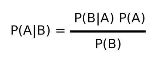
Conditional Probability... Again, the probability of an event given that another event has occurred is called a conditional probability...

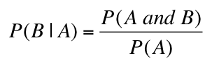 Note how “A given B” and “B given A” are related...
1% of women have breast cancer: P(BC)=0.01
80% of mammograms detect breast cancer when it is there : P( MP | BC ) = 0.8
9.6% of mammograms detect breast cancer when it’s not there : P( MP | BCc ) = 0.096
What’s the probability of having breast cancer given that mammogram detected breast
cancer? P ( BC | MP )
Historically, your asking out a girl for a date was successful with 40%. New information: You fancy a girl and she smiled at you today. Historically, among the girls who accepted when you ask out, 60% smiled before. Among the girls who rejected, 20% of girls smiled before. What’s the chance that asking out your crush is accepted?
-
● Let B = accepted, Bc = rejected -
● P(B)=0.4,P(Bc )=0.6 -
● Define the smile event as A -
● Conditional probabilities: P(A|B) = 0.6 P(A|Bc ) = 0.2 -
● Goal is to find P(B|A)
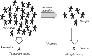
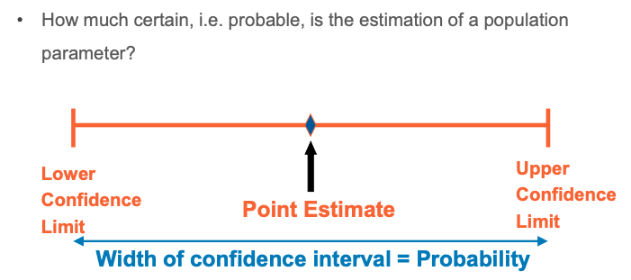
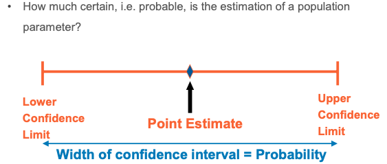
To estimate the mean value(μ) from sample mean (𝑿)
- How confident you are of the estimated value?
- Confidence interval To test a hypothesis (H0) from sample - How probable the hypothesis is?
- Significant level

Statistics and Probability
-
Assume that you got 175 cm of average height from the sample.
-
Probably you’d like to mention that the average height of the population would be 175 cm.
-
How confident are you when you mention it? What’s the probability of μ being 175 cm
Source: https://medium.com/@garora039/what-exactly-is-central-limit-theorem-7c1531eb2987/
-
Assume that gambler bet $1 for a head and you bet $1 for a tail
-
The gambler won the game, would you be suspicious about the fairness of the coin?
-
What if you lost the game 10 times straight?
Probability and Statistics

Source: http://thai-massagen.com/?page_id=6120
Variable and probability distribution Assume a situation that we flip a coin twice.
Variable X: # of Tails
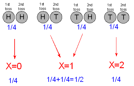
Probability Distribution Table
Probability Distribution Graph
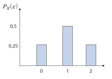
Probability distribution
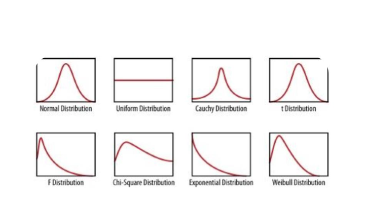
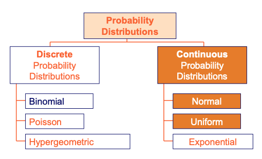
Probability Distributions
-
Binomial distribution
-
Poisson distribution
-
Z distribution (gaussian, normal) - t distribution
-
F distribution, χ2 distribution
Source: https://medium.com/analytics-vidhya/probability-distributions-444e7babf2e1
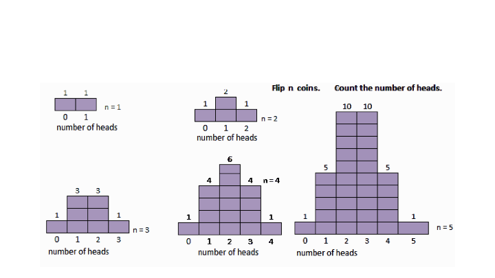
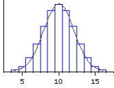
Binomial Distribution Variable: # of Heads when flipping coin 4 times
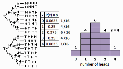
Variable: # of Heads when flipping coin n times
Random Variable: # of Heads when flipping coin 20 times
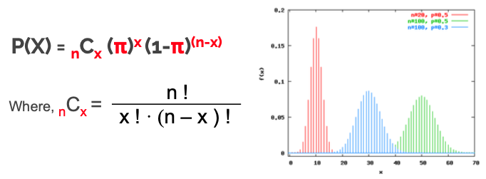
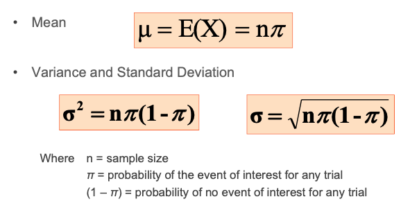
Assume that the probability of having heads is π, not 0.5 due to certain reason. Then the probability that we have X times of heads(π) when flipping n times
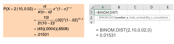
Binomial Distribution Example
-
Suppose the probability of purchasing a defective computer is 0.02.
-
What is the probability of purchasing 2 defective computers in a group of 10?
➔n = 10, x = 2, p = 0.02
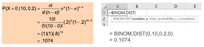
Binomial Distribution Example
-
What’s the probability of getting zero score when you select the answer randomly?
-
You got 10 multiple choice questions, and each of them has 5 answers ➔n = 10, x = 0, π = 0.2
-
If a grade on the exam is less than 50, that’s considered a failed
-
What’s the probability of getting failed? ➔ Given that n=10 and π = 0.2 P(fail quiz) = P(X < 4) = P(0)+P(1)+P(2)+P(3)+P(4) This is called a cumulative probability, that is, P(X ≤ x)
= BINOM.DIST(4,10,0.2,1) = 0.9672

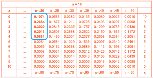
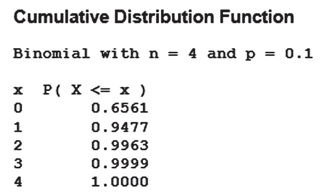
Binomial Distribution Table
• P(fail quiz) = P(X < 4) = P(0)+P(1)+P(2)+P(3)+P(4)
= 0.1074+0.2684+0.3020+0.2013+0.0881 = 0.9672
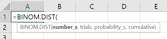
Using Excel
• Use the Excel function, “BINOM.DIST”, • BINOM.DIST(4,10,0.2,1)
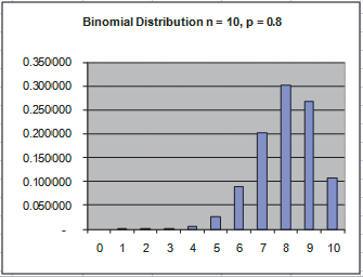
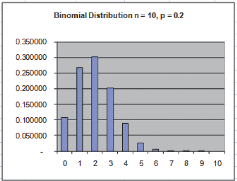
Shapes of Binomial Distribution
• The shape of the binomial distribution depends on the values of π and n
Positively skewed when π (or p) < 0.5
Positively skewed when π (or p) > 0.5
Binomial Distribution Characteristics
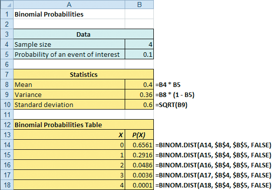
Binomial Distribution in Excel
• When n=4 and π=0.1
Binomial Distribution in Excel
-
Suppose that 15% of people are left-handed.
-
What is the probability of finding exactly 9 left-handed people in a random sample of 50? ➔ Using Excel’s BINOM.DIST function, the answer is =BINOM.DIST(9, 50, 0.15, FALSE) = 0.1230
Binomial Distribution – Conditions and Criteria
-
Rule 1: Situation where there are only two possible mutually exclusive outcomes (for example, yes/no survey questions).
-
Rule2: A fixed number of repeated experiments and trials are conducted (the process must have a clearly defined number of trials).
-
Rule 3: All trials are identical and independent (identical means every trial must be performed the same way as the others; independent means that the result of one trial does not affect the results of the other subsequent trials).
-
Rule: 4: The probability of success is the same in every one of the trials.
-
Source: http://www.intellspot.com/binomial-distribution-examples/
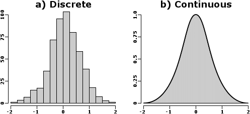
Probability Distributions
Continuous Probability Distribution
-
Computing probabilities from the normal distribution
-
Using the normal distribution to solve real world problems
-
Computing probabilities from the uniform distribution
-
A continuous random variable is a variable that can assume any value on a continuum ✓ thickness of an item ✓ time required to complete a task ✓ temperature ✓ height, weight
-
Continuous probability distributions can have a variety of shapes
-
Two common continuous distributions
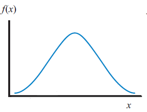
Normal Distribution
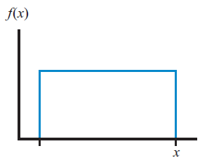
Uniform Distribution
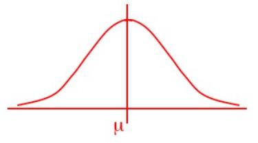
The Normal Distribution
-
Bell Shaped, Symmetrical (Mean, Median and Mode are Equal)
-
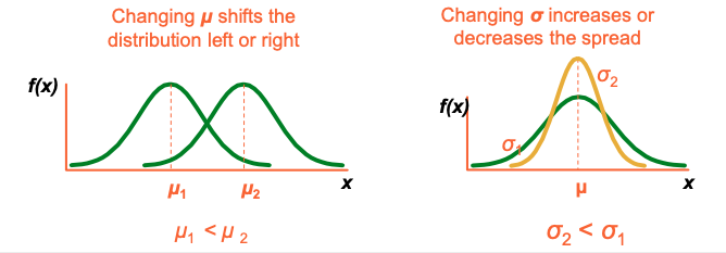
Location is determined by the mean, μ
-
Spread is determined by the standard deviation, σ
-
The random variable has an infinite theoretical range f(X)
μ
Mean = Median = Mode
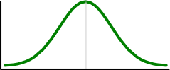
The Normal Distribution Shape
• A distribution’s mean (μ) and standard deviation (σ) completely describe its shape
The Normal Distribution • The Normal Probability Density Function:
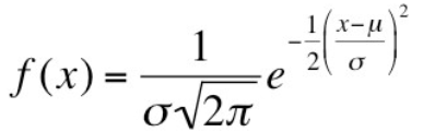
✓ e : Euler number, 2.71828...... ✓ π : ratio of a circle's circumference to its diameter,3.14159...... ✓ μ : the mean of the distribution ✓ σ : the standard deviation of the distribution ✓The range of random variable x: ∞<x<∞
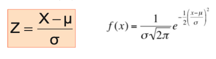
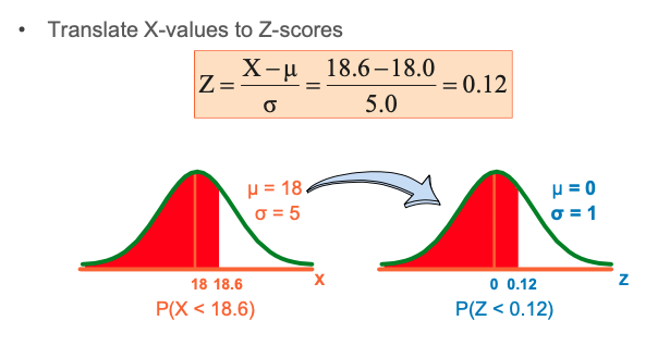
Translation to the Standardized Normal Dist.
• Translate from X to the standardized normal (the “Z” distribution) by subtracting the mean of X and dividing by its standard deviation:
Translation to the Standardized Normal Dist
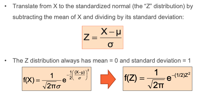
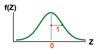
The Standardized Normal Distribution
-
Also known as the “Z” distribution
-
Mean is 0
-
Standard Deviation is 1
Example
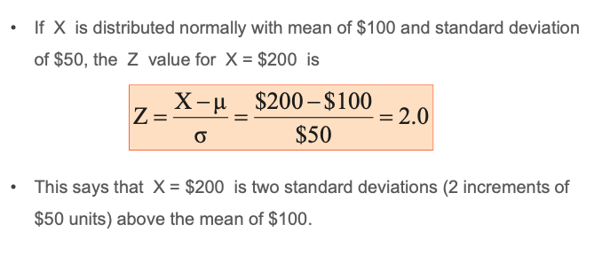
Comparison of the X and Z value
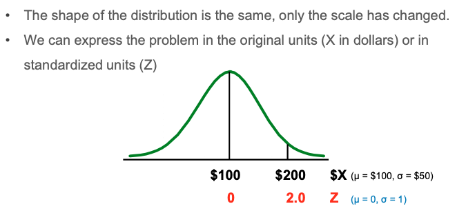
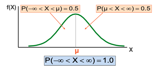
Probability as Area Under the Curve
• The total area under the curve is 1.0, and the curve is symmetric, so half is above the mean, half is below
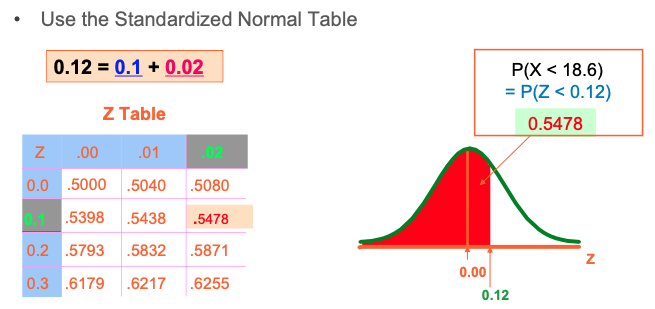
Procedure for Finding Normal Probabilities
- To find P(a < X < b) when X is distributed normally: Draw the normal curve for the problem in terms of X Translate X-values to Z-scores Use the Standardized Normal Table Use Excel function
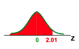
Probability as an area
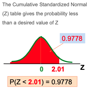
What will be the probability of P(Z <2.01)?
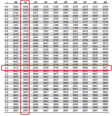
Z Table
Excel function
-
- norm.dist(x, mean, standard deviation, cumulative) -
- norm.inv(probability, mean, standard deviation) -
- norm.s.dist(z, cumulative) - norm.s.inv(distribution)
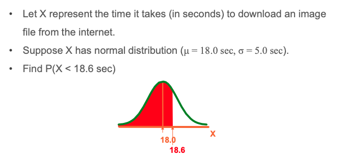
Example - Finding Normal Probabilities
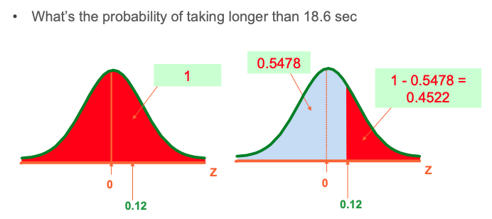
Finding Normal Upper Tail Probabilities
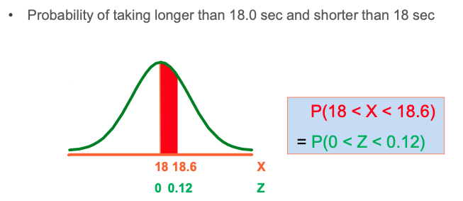
Normal Probability Between Two Values
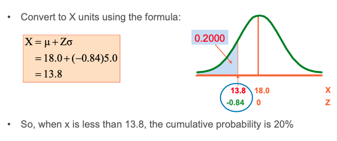
Finding the X value for a Known Probability
-
X represent the time it takes to download an image file from the internet.
-
Suppose X has normal distribution (μ = 18.0 sec, σ = 5.0 sec).
-
Find X such that 20% of download times are less than X.
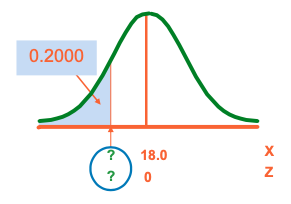
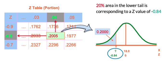
Find the Z value for 20% in the Lower Tail
• Find the closest Z value for the known probability (20%)
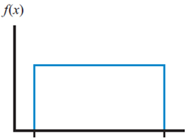
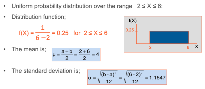
The Uniform Distribution
• The uniform distribution is a probability distribution that has equal probabilities within a certain range
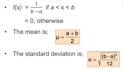
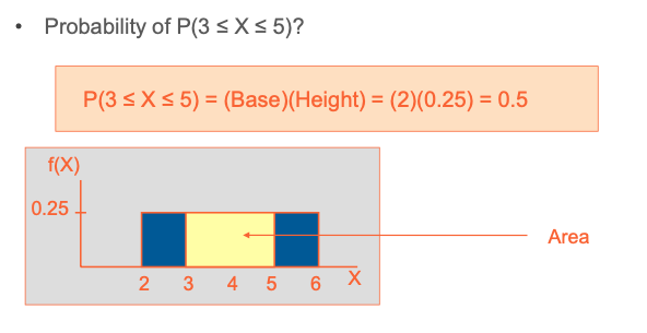
Example - The Uniform Distribution
Sample distribution and Confidence interval
- Sampling distribution
- Central Limit Theorem
- Confidence interval of population mean
- ( Z distribution / t distribution )
Statistical Inference
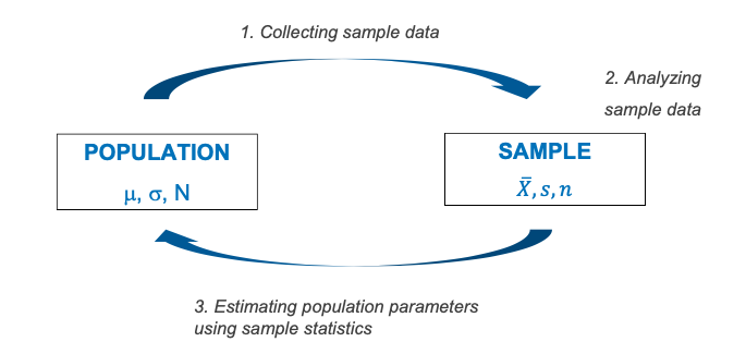
Mathematical Notation
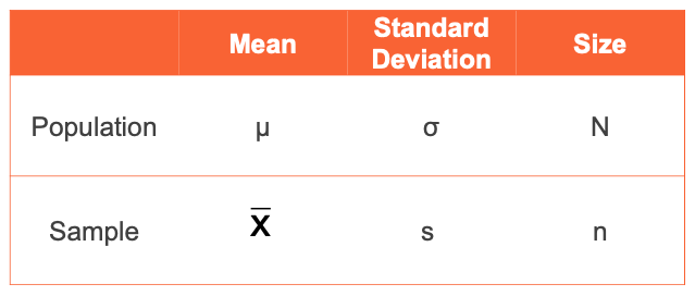
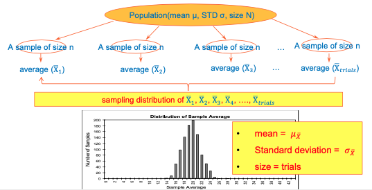
Distribution of sample mean
- Sample mean (𝑋) changes when you take different sample
- How would sample mean (𝑋) be distributed then?
Mathematical Notation
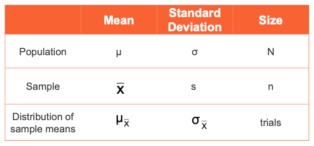
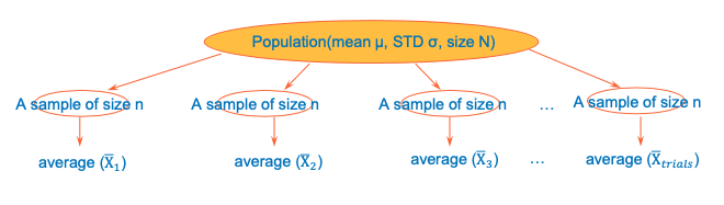
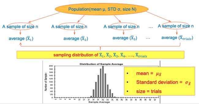
Distribution of sample mean

Sample distribution
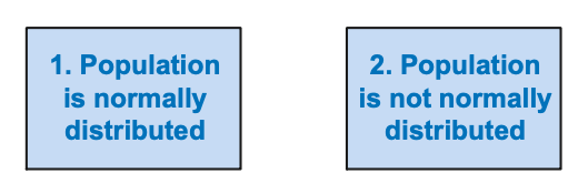
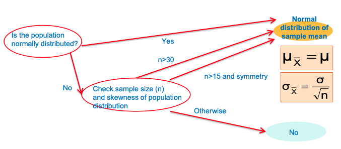
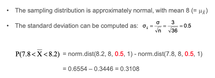
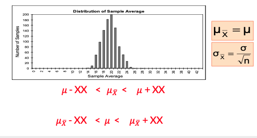
Sample distribution – when the population is normally distributed
-
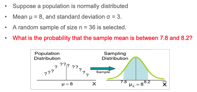
If a population is normal with mean μ and standard deviation σ,
-
The sampling distribution of 𝑥ҧ is also normally distributed with
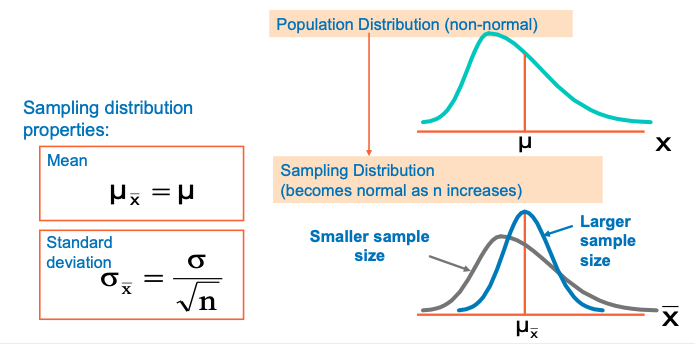
Central Limit Theorem
-
Even if the population is not normal,
-
Sample means from the population will be approximately normal as long as the sample size is large enough.
-
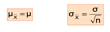
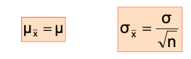
Properties of the sampling distribution of 𝑥ҧ :
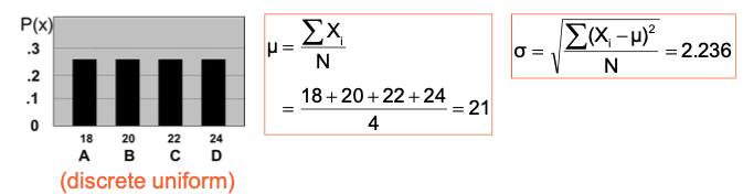
Example - a Sampling Distribution
-
Assume there are 4 people (N = 4)
-
Random variable, X, is age of individuals (X: 18, 20, 22, 24 years old)
-
Summary measures for the population distribution
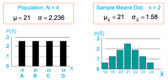
Distribution of sample mean
Example
Solution – using excel function (norm.dist)
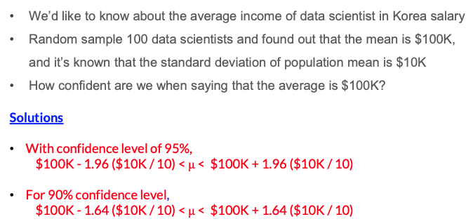
Confidence interval of the population mean
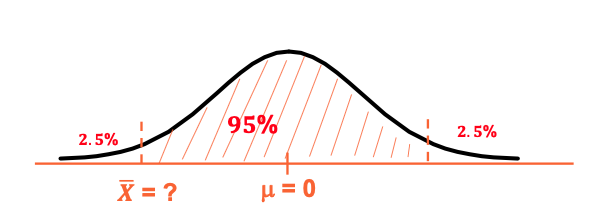
Standard Normal Distribution
-
Normal distribution with = 0, = 1 ത
-
What’s the 𝑋 value where the probability of dashed are is 95%?
-
norm.inv(0.025,0,1) = -1.96, norm.inv(0.975,0,1) = 1.96
-
95% confidence interval for 𝑋
-1.96 ≤ 𝑋 ≤ 1.96
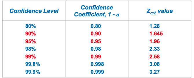
Normal Distribution: Critical Z-Scores
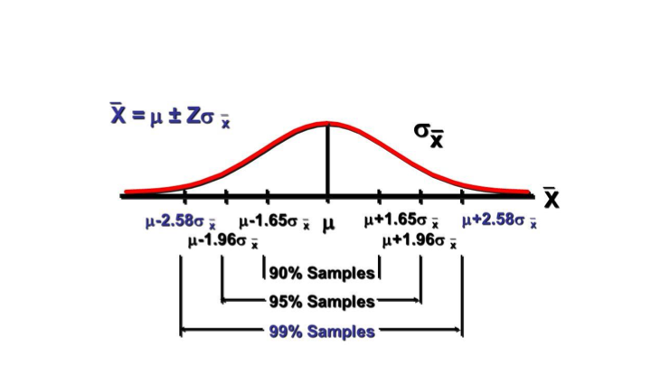
Common levels of confidence
- Commonly used confidence levels are 90%, 95%, and 99%
Confidence Interval for Population Mean (when population STD(σ) is unknown)
-
If the population standard deviation σ is unknown, we can substitute the sample standard deviation, s
-
This introduces extra uncertainty, since s varies from sample to sample
-
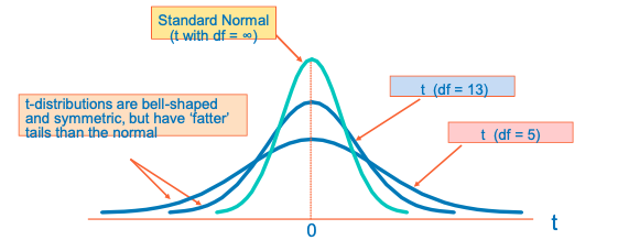
So we use the Student’s t distribution instead of the normal distribution ✓ The t distribution allows more uncertainty than normal when the degree of freedom is low ✓ The tα/2 value depends on degrees of freedom (d.f.) ✓ Degrees of freedom (d.f.) is identified as ‘n-1’
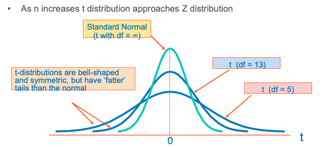
Student’s t Distribution
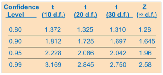
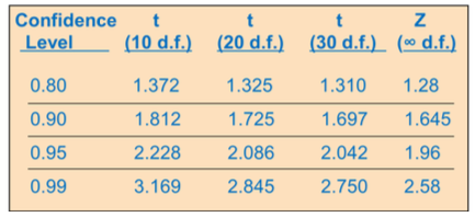
A few selected t distribution values
With comparison to the Z value (degree of freedom = sample size -1)
(you can also get the number from excel function “t.inv.2t(probability, d.f.)”
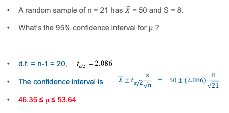
Example of t distribution confidence interval
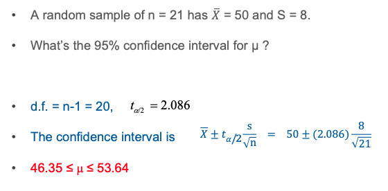
Confidence interval of the population mean
Confidence Interval for Population Mean (when population STD(σ) is unknown)
-
If the population standard deviation σ is unknown, we can substitute the sample standard deviation, s
-
This introduces extra uncertainty, since s varies from sample to sample
-
So we use the Student’s t distribution instead of the normal distribution The t distribution allows more uncertainty than normal when the degree of freedom is low The tα/2 value depends on degrees of freedom (d.f.) Degrees of freedom (d.f.) is identified as ‘n-1’
Student’s t Distribution
• As n increases t distribution approaches Z distribution
A few selected t distribution values
• With comparison to the Z value (degree of freedom = sample size -1)
(you can also get the number from excel function “t.inv.2t(probability, d.f.)”
Example of t distribution confidence interval
- Hypothesis test – Z test, t test Critical value and p-value
- One-tail test and two-tail test Type I, II error
Hypothesis Testing
- While you’re traveling, you met a gambler
- He bet $1 for a head, and me bet $1 for a tail
- He won the game 7 times straight
- You claim that the coin is not a normal one
- But he argued that it was an absolute coincidence, nothing’s impossible in the probability distribution How would you argue?
Hypothesis testing is a process of testing the hypothesis with pre- defined confidence level
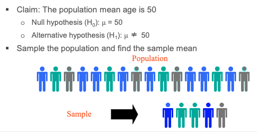
- A hypothesis is a claim about a population parameter (e.g. mean)
- Sample mean is estimated
- Checks whether the sample mean is within the confidence interval from the claimed mean (i.e. the hypothesis)
Terminology
- Null hypothesis (H0): a claim to be test
- Alternative hypothesis (H1): the opposite of the null hypothesis
- Significance level: interval for the rejection (α)
- Confidence level: interval for the acceptance of the H0, ( (1- α) x 100% )
- Confidence level = (1 – α ) x 100%
- Confidence coefficient = 1 – α
- Level of Significance (probability corresponding to 2 tail) = α
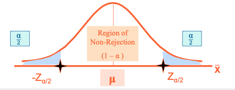
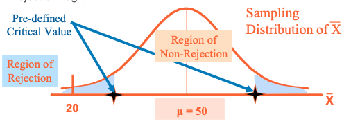
Hypothesis Testing Process
- Suppose the sample mean age was 20, (𝑋 = 20)
- Check where the sample mean falls on (1) rejection region, (2) non- rejection region
Hypothesis Testing – Example 1
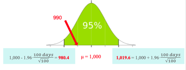
- A manufacturer claims that the average lifetime of a light bulb is 1,000days. (standard deviation: 100days)
- An inspector found that the sample mean of 100 bulbs is 990 days
- Test null hypothesis (H0: life-time is 1,000 days) with 5% of significance level (i.e. α = 0.05)
Hypothesis Testing – Example 1 (x value)
- H0 are not rejected as the 𝑋 value is within the interval
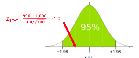
Hypothesis Testing – Example 1 (z value)
- You can check the region with ZSTAT value
Hypothesis Testing – Example 1 (p value)
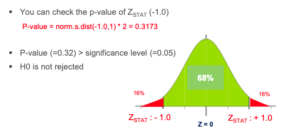
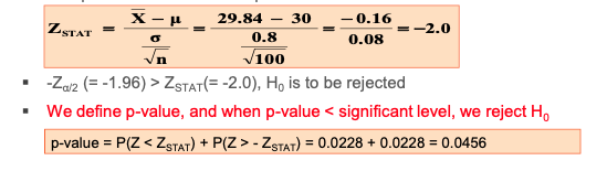
Hypothesis Testing – Example 2 (p-value)
-
A manufacturer claims that the mean diameter of a manufactured bolt is 30mm. (Assume σ = 0.8)
-
Test the claim with significant level of 5%
-
Sample mean from 100 samples was 29.84
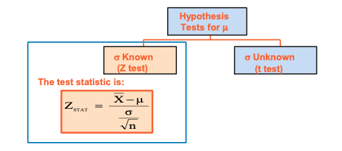
Hypothesis Testing when σ is known
- Z-Test is used when the population standard deviation is known
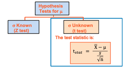
Hypothesis Testing when σ is unknown
- t-Test is used when the population standard deviation is unknown
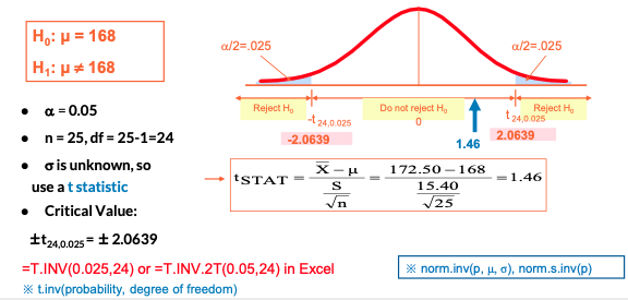
Hypothesis Testing – Example 3 (t-test)
- The average price of a hotel room in NY is said to be $168 per night.
- A random sample of 25 hotels is taken, 𝑋 = $172.50 and s = $15.40.
- Test null hypothesis with 5% of significance level (i.e. α = 0.05)
One-Tail Tests
- In many cases, the hypothesis focuses on a particular direction
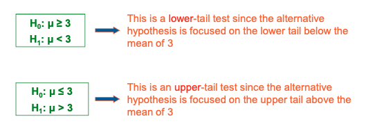
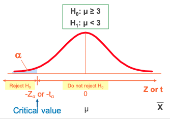
Lower-Tail Tests
- There is only one critical value, since the rejection area is in only one tail
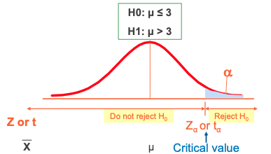
Upper-Tail Tests
There is only one critical value, since the rejection area is in only one tail
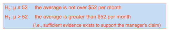
Upper-Tail Tests ( unknown) - Example
- Average of the monthly cell phone bills is known to be $52 per month
- A phone industry manager thinks that it has increased, and wishes to test this claim.
- Suppose that α = 0.10, n=25 is chosen for this test
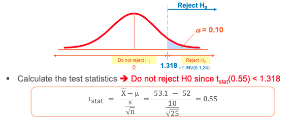
- From the 25 samples (n = 25), we’ve got 𝑋 = 53.1, s = 10.
Upper-Tail Tests ( unknown) - Example
- Finding the rejection region:
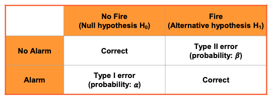
Type I, II Errors
There are possible errors in hypothesis test decision making
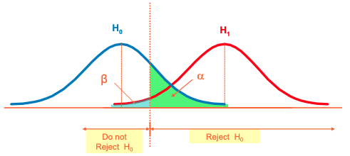
Type of Errors in Hypothesis Test

Linear Relationship
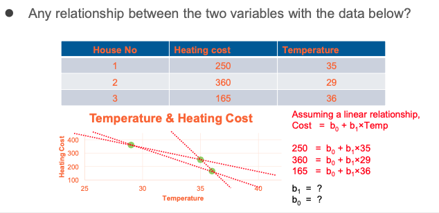
Introduction to Regression Analysis
- Dependent variable:
- The variable we wish to predict or explain (e.g. heating cost)
- Typical symbol is Y.
- Independent variable(s):
- The variable used to predict or explain the dependent variable.
- E.g. temperature, insulation, age of boiler, number of windows
- Typical symbol is X.
Introduction to Regression Analysis
- Regression analysis is used for:
- Explaining the impact of changes in independent variable(s) on the dependent variable.
- Predicting the value of a dependent variable based on the value of independent variable(s).
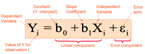
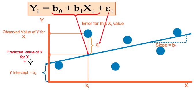
Simple Linear Regression Model
- Only one independent variable, X
- Changes in Y are assumed to be related to changes in X
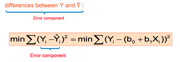
The Least Squares Method
- b0 and b1 are obtained by minimizing the sum of the squared
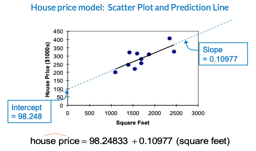
Simple Linear Regression Example
- A real estate agent wishes to examine the relationship between the selling price of a home and its size (measured in square feet)
- A random sample of 10 houses is selected
- Dependent variable (Y) = house price in $1000s
- Independent variable (X) = square feet
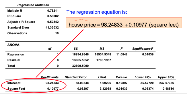
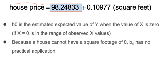
Simple Linear Regression Example: b0
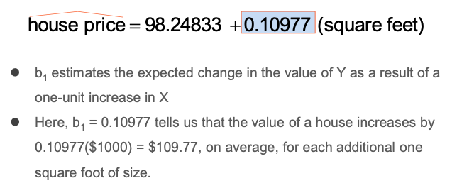
Simple Linear Regression Example: b1
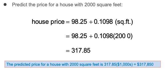
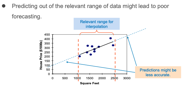
Simple Linear Regression Example: Prediction
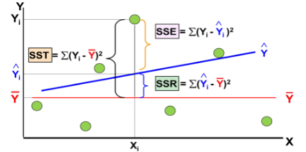
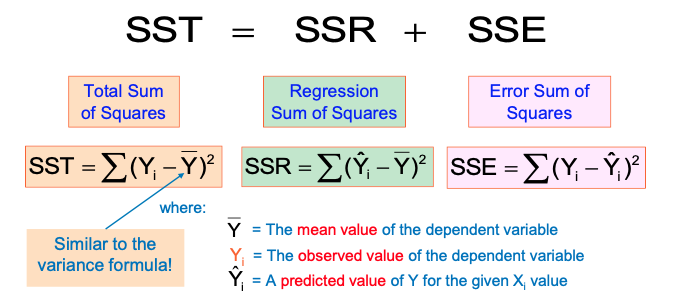
Model Evaluation: Measures of Variation
- SST = total sum of squares (Total Variation)
- SSR = regression sum of squares (Explained Variation)
- SSE = error sum of squares (Unexplained Variation)
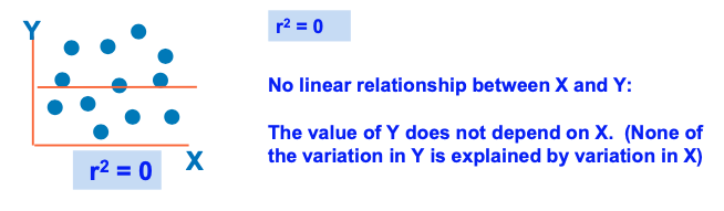
Simple Linear Regression Example: R2
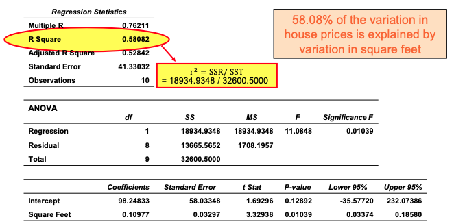
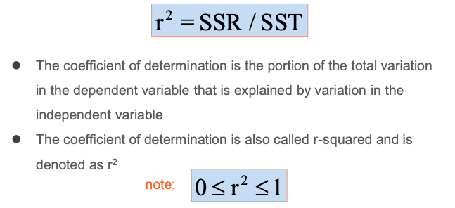
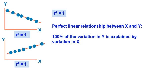
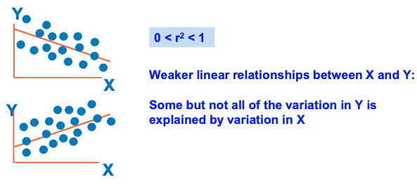
Coefficient of Determination: R2
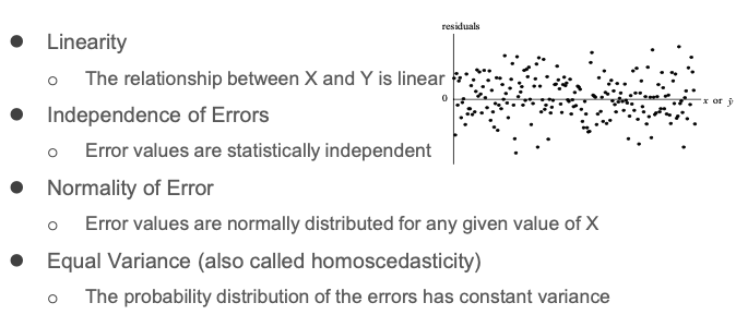
Regression Diagnostics (L.I.N.E)
Multiple Regression
- Often we can obtain more accurate forecasts if we include more independent variables in our regression model.
- Example) heating cost would be affected by not only the size but, temperature, insulation, age of boiler, number of windows as well.
- Allows effect of changes in some variables to be investigated while others are held constant.
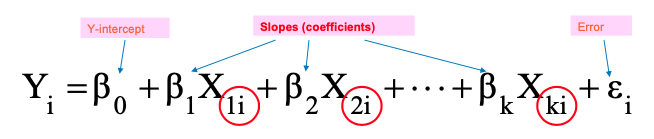
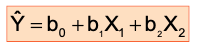
Multiple Regression Model
- Idea: Examine the linear relationship between 1 dependent (Yi) and 2 or more independent variables (Xi)
- Multiple Regression Model with k Independent Variables:
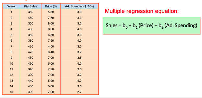
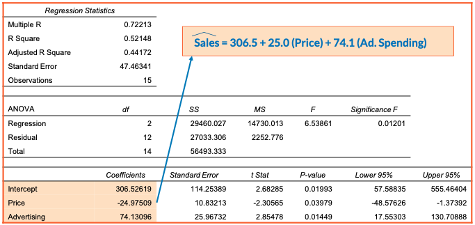
Example: two Independent Variables
- A distributor of frozen dessert pies wants to evaluate factors thought to influence demand
- Dependent variable: Pie sales (units per week) o Independent variables: Price (in $) Advertising ($100’s)
- Data are collected for 15 weeks
Example: two Independent Variables
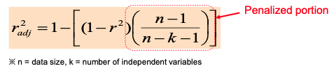
R2 vs. Adjusted R2
- r2 never decreases even if an irrelevant new X variable is added to the model
- This can be a disadvantage when comparing models
Adjusted r2
- Penalize when adding a new variable
- If the new variable is very useful, adjusted r2 will still increase
Using Dummy Variables
- A dummy variable is a categorical independent variable with two levels:
- yes or no, on or off, male or female
- If more than two levels, (number of levels - 1) number of dummy
variables are needed.
- Spring, summer, fall, winter 3 dummy variables are needed
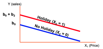
Dummy-Variable Example
- Let the regression model be
- Y = pie sales per week
- X1 =pricein$
- X2 = holiday ( b2 = 1 if a holiday occurred during the week, 0 otherwise)
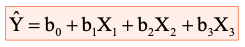
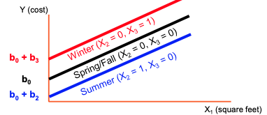
Dummy-Variable Example (more than 2 levels)
- Let the regression model be
- Y = heating cost
- X1 = square feet
- X2 = 1 if summer, X3 = 1 if winter, (spring/fall be the default category)
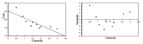
Nonlinear Relationships
- Plots show we are fitting a linear model to a relationship that is non- linear (e.g. cost vs capacity).
- If there is a pattern in residuals, we have missed something.
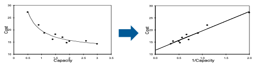
Nonlinear Relationships
- Non-linear relationship can be transformed to linear relationship using ‘1/capacity’ instead of ‘capacity’
- After the transformation, the adjusted r2 increases
The problem of multicollinearity
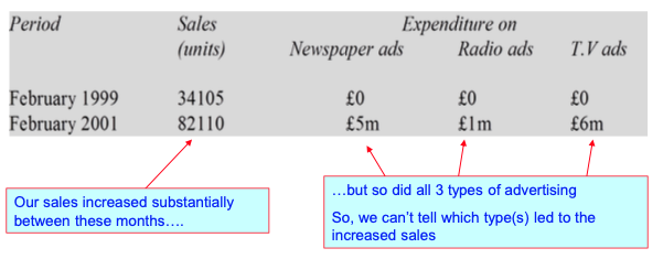
The problem of multicollinearity
- Occurs when there’s high correlation between the independent variables.
- Independent variables contribute redundant information to the model.
- Problems:
- The coefficients estimated cannot be trusted.
- The coefficients might even have the wrong signs.
- Indications:
- Intuitively Incorrect signs on the coefficients.
- When a new variable is added to the model, there’s a large change in the value of a previous coefficient.
Detecting and solution to the multicollinearity
- Run a separate regression with one suspicious variable as dependent and all the others as independent variables.
- If r2 > 0.8, then it’s regarded as there’s a multicollinearity issue
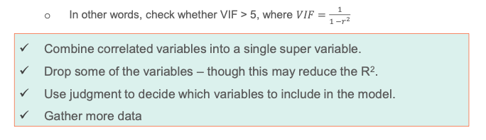
- If r2 > 0.8, then it’s regarded as there’s a multicollinearity issue