DATA 410 Advanced Applied Machine Learning Midterm Project

In this project, we will apply the linear Generalized Additive Model and the Nadaraya-Watson kernel density estimator to the CASP.csv data set. We will use the R-squared coefficient and the Residual Mean Squared Error obtained from a 10-fold cross validation process to compare the performance of the two methods. At the end of the project, we will include residual plots and histograms for results from both train and test split.

General Imports

These imports are the tools for regularization techniques, hyperparameter tuning, and 5-Fold validation process.

!pip install pygam

import numpy as np
import pandas as pd
from pygam import LinearGAM
from sklearn.model_selection import train_test_split as tts
from sklearn.model_selection import KFold
from sklearn.preprocessing import StandardScaler
from sklearn.metrics import mean_squared_error as MSE
from sklearn.metrics import r2_score as R2_Coef
import matplotlib.pyplot as plt
from scipy.optimize import minimize
from matplotlib import pyplot
from nadaraya_watson import NadarayaWatson, NadarayaWatsonCV

Data Processing

When applying the Nadaraya-Watson kernel density estimator, we found that the dataset has too many observations and there is not enough RAM for Google Colab to perform a complete kernel estimation. As a result, we randomly dropped 40000 observations and applied the kernel estimator on the rest 5730 obervations.

df = pd.read_csv('/content/CASP.csv')
df = df.drop(np.random.choice(range(45730),size=40000,replace=False))
features = ['F1','F2','F3','F4','F5','F6','F7','F8','F9']
X = np.array(df[features])
y = np.array(df['RMSD']).reshape(-1,1)
Xdf = df[features]

For the linear Generalized Additive Model, Google Colab is powerful enough to take all 45730 observations. So, we did not remove any part of the data set.

Generalized Additive Model

The generalized Additive Model (GAM) is a generalized linear model in which the linear response variable depends linearly on unknown smooth functions of some predictor variables. Similar to linear regression process where we estimate for beta coefficients, we try to estimate the unknown functions associated with the predictor variables in GAM.

Importing the data set:

df = pd.read_csv('/content/CASP.csv')
features = ['F1','F2','F3','F4','F5','F6','F7','F8','F9']
X = np.array(df[features])
y = np.array(df['RMSD']).reshape(-1,1)
Xdf = df[features]

10-Fold Cross Validation Process:

def DoKFold_GAM(X,y,rs,n_splines):
  PE_external_validation = []
  R2_coefficient = []
  kf = KFold(n_splits=10,shuffle=True,random_state=rs)
  for idxtrain, idxtest in kf.split(X):
    X_train = X[idxtrain,:]
    y_train = y[idxtrain]
    X_test = X[idxtest,:]
    y_test = y[idxtest]
    gam = LinearGAM(n_splines=n_splines).gridsearch(X_train, y_train,objective='GCV')
    yhat_test = gam.predict(X_test)
    PE_external_validation.append(MSE(y_test,yhat_test,squared=False))
    R2_coefficient.append(R2_Coef(y_test,yhat_test))
  return np.mean(PE_external_validation), np.mean(R2_coefficient)

Since there are 45730 observations, the least number of splines is 23.

DoKFold_GAM(X,y,1693,23)

(4.919868824649355, 0.35297175269122966)

The GAM with 23 splines yields a RMSE of 4.919868824649355 and a R-squared coefficient of 0.35297175269122966.

Nadaraya-Watson Kernel Density Estimator

Nadaraya and Watson, both in 1964, proposed to estimate for a dependent variable as a locally weighted average, using a kernel as a weighting function. One advantage of this method is that it is not affected by the values of the predictor variables.

10-Fold Cross Validation Process:

def DoKFold_kernel(X,y):
  PE = []
  R2_coefficient = []
  kf = KFold(n_splits=3,shuffle=True,random_state=1693)
  for idxtrain, idxtest in kf.split(X):
    param_grid=dict(kernel=["laplacian"],gamma=np.logspace(-5, 5, 20))
    model = NadarayaWatsonCV(param_grid,scoring='neg_mean_absolute_error')
    X_train = X[idxtrain,:]
    y_train = y[idxtrain]
    X_test  = X[idxtest,:]
    y_test  = y[idxtest]
    model.fit(X_train,y_train)
    yhat_test = model.predict(X_test)
    PE.append(MSE(y_test,yhat_test,squared=False))
    R2_coefficient.append(R2_Coef(y_test,yhat_test))
  return np.mean(PE), np.mean(R2_coefficient)

Calling the function:

DoKFold_kernel(X,y)

(6.294144531698417, -0.05344013234906527)

The Nadaraya-Watson kernel density estimator yields a RMSE of 6.294144531698417 and R-squared coefficient of -0.05344013234906527. In comparison with the GAM method, the kernel estimator has a worse performance, especially in terms of R-squared coefficient. A negative R-squared value means that the model is worse than a constant function, which has a R-squared value of 0.

Visual Representation

Generalized Additive Function

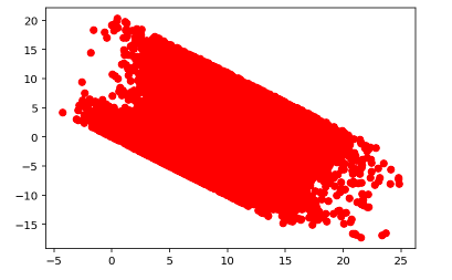
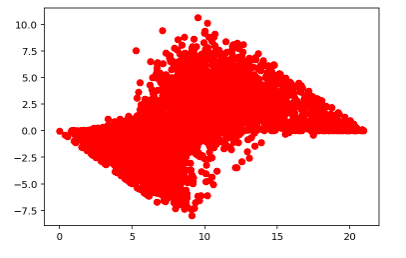
Residual vs Fitted Values for Train Data

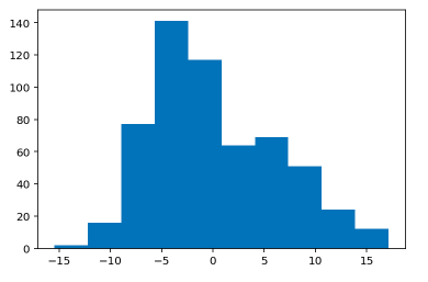
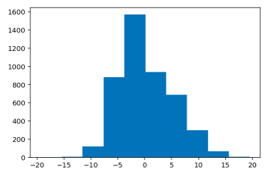
Histogram of Train Residual Values

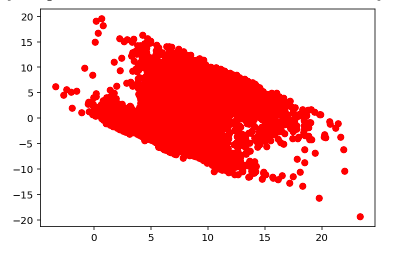
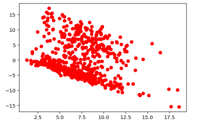
Residual vs Fitted Values for Test Data

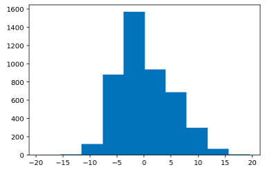
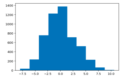
Histogram of Test Residual Values

Nadaraya-Watson Kernel Density Estimator

Residual vs Fitted Values for Train Data

Histogram of Train Residual Values

Residual vs Fitted Values for Test Data

Histogram of Test Residual Values