#stat4701-edav-d3.github.com

COMMIT TEST - Danny

###LIVE PROJECT WEBSITE ####The GitHub Project Website Repo ####The GitHub Project Folder #####The GitHub Organization

#To Do:

• Grab city's from Table - create a list of city's
• geocode that list
• create shapefile of that list
• create geojson of cities list with coords and Flu Data
  • maybe all good on this, see cities ... html

http://bost.ocks.org/mike/bubble-map/base.html

#Outline for Remark Presenation

Code below this point will be pasted into the Remark html

---

Stephen and Danny's D3 Mapping Presentation

from Shapefile to TopoJSON (and some GeoJSON) using GDAL/OGR

---

Agenda

1. Introduction
2. Flu Data
3. D3 Examples and Inspiration

X. Maybe a demo that people can follow to do a very basic d3 map (maybe not, seems like this browser issues and others could be a huge pain) X. Maybe do something with CartoDB at the end. If no one else is talking about it, it could be useful to at least mention and show a few things.

---

Introduction

some code

---

Data

##CDC

###Scraping and Munging CDC Flu Data in R

library(cdcfluview)
library(dplyr)
library(magrittr)
library(ggplot2)

dat <- get_flu_data(region="hhs", 
                sub_region=1:10, 
                data_source="ilinet", 
                years=2000:2014)

dat %<>%
  mutate(REGION=factor(REGION,
                   levels=unique(REGION),
                   labels=c("Boston", "New York",
                            "Philadelphia", "Atlanta",
                            "Chicago", "Dallas",
                            "Kansas City", "Denver",
                            "San Francisco", "Seattle"),
                   ordered=TRUE)) %>%
mutate(season_week=ifelse(WEEK>=40, WEEK-40, WEEK),
     season=ifelse(WEEK<40,
                   sprintf("%d-%d", YEAR-1, YEAR),
                   sprintf("%d-%d", YEAR, YEAR+1)))

prev_years <- dat %>% filter(season != "2014-2015")
curr_year <- dat %>% filter(season == "2014-2015")

curr_week <- tail(dat, 1)$season_week

gg <- ggplot()
gg <- gg + geom_point(data=prev_years,
                  aes(x=season_week, y=X..WEIGHTED.ILI, group=season),
                  color="#969696", size=1, alpa=0.25)
gg <- gg + geom_point(data=curr_year,
                  aes(x=season_week, y=X..WEIGHTED.ILI, group=season),
                  color="red", size=1.25, alpha=1)
gg <- gg + geom_line(data=curr_year, 
                 aes(x=season_week, y=X..WEIGHTED.ILI, group=season),
                 size=1.25, color="#d7301f")
gg <- gg + geom_vline(xintercept=curr_week, color="#d7301f", size=0.5, linetype="dashed", alpha=0.5)
gg <- gg + facet_wrap(~REGION, ncol=3)
gg <- gg + labs(x=NULL, y="Weighted ILI Index", 
            title="1999-2015 Weighted Flu Index by CDC Region; Week Ending Jan 3, 2015 (Current Season in Red)n")
gg <- gg + theme_bw()
gg <- gg + theme(panel.grid=element_blank())
gg <- gg + theme(strip.background=element_blank())
gg <- gg + theme(axis.ticks.x=element_blank())
gg <- gg + theme(axis.text.x=element_blank())
gg

##Google Flu Trends

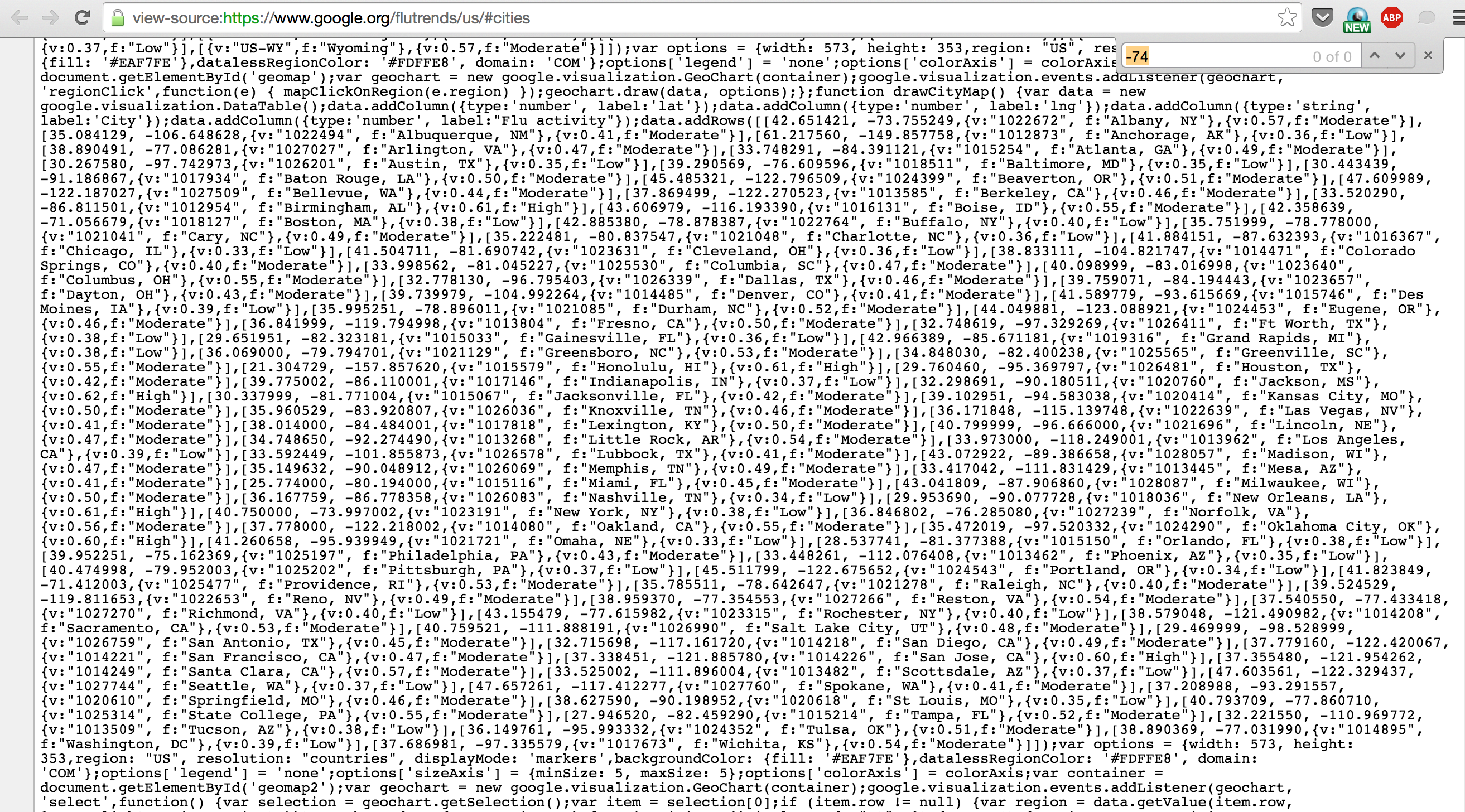
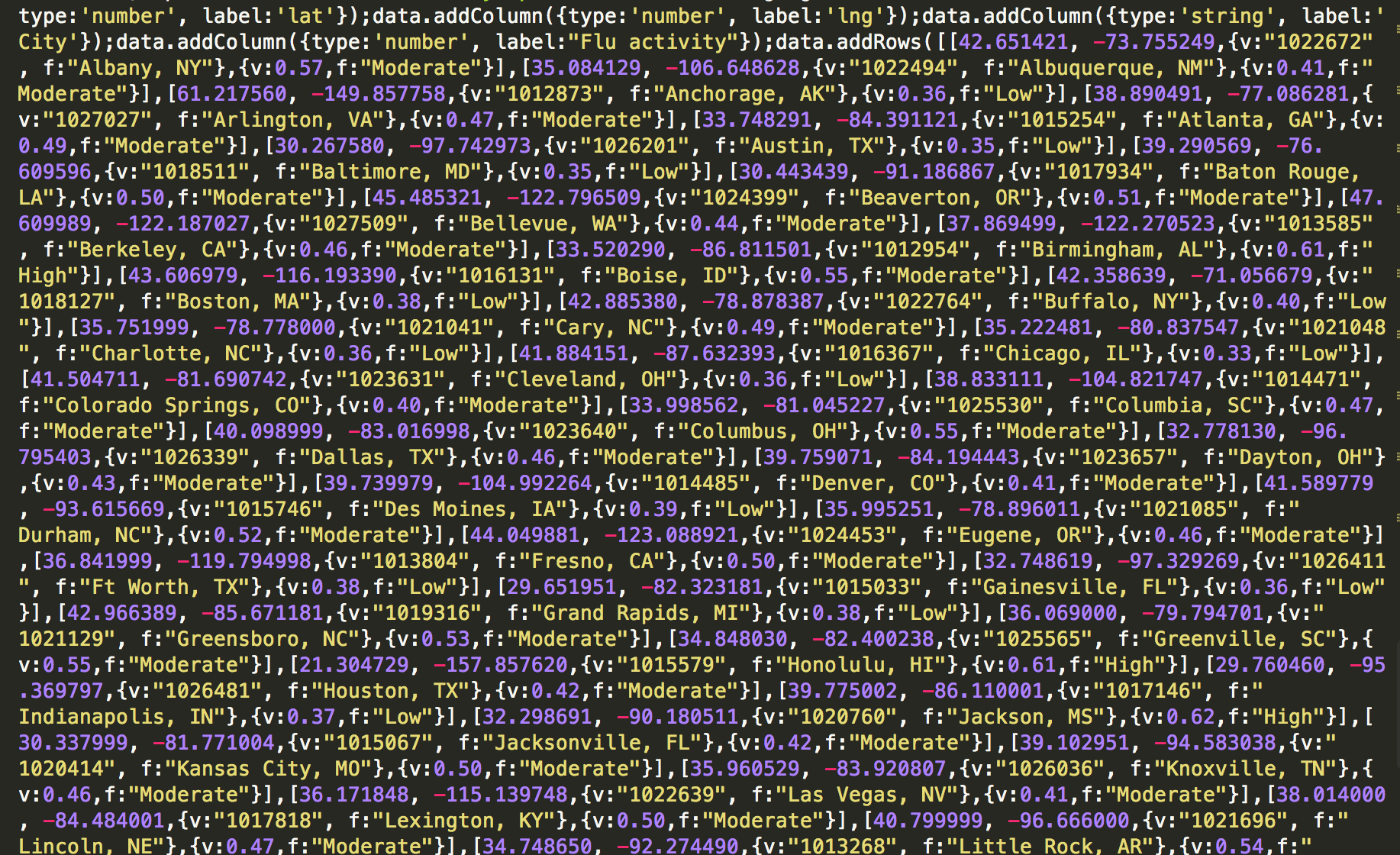
###Cities Lat/Longs

---

What's not cool about D3

some code