Meteorological Data Quality Assesment (UNDER DEVELOPMENT)

Open-source Python implementation of a quality control system for meteorological data.

The context of this master thesis is DMI's NCKF (National Center for Climate Research) DANRA project [@DANRA]. The input data used in DANRA and for development purposes of this project includes in-situ observation of multiple variables (pressure, temperature, visibility, precipitations ...) However the aim of the project is to develop a framework which can be applied to any meteorological database without extensive modifications.

Before those measurements enter systems for assimilation, it is necessary to asses the quality of the latter to avoid potentially errorneous information due to different reasons such as biases or other instrument errors.

For achieving these objectives, of course it is impossible to compare the measurements to the true values that we are precisely trying to measure. However, the discrepancy and correction can be estimated by comparing our measurements to others in the database and use some gross assumptions about the coherence of the values:

• Coherence in space: In the physical system that we are describing, measurements have to be correlated within the distance. This means that the closer the measurements are within each other, the more correlated they have to be. This is general though and some comments have to be made. The spatial coherence is also affected by other factors than the distance, for example the orography of the surface where the stations are placed. If two stations are placed within a flat surface, for example a valley, their correlation will be different than if they are placed within a mountain. Other aspects that could affect the correlation are atmospheric conditions such as air pressure.

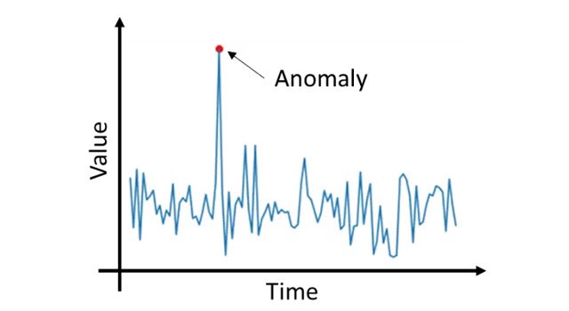
• Coherence in time: The measurements of a single station can be represented in the form of time series. In overall the station network can be seen as a multivariate time series. This series carry trends, features and periodicity whose description is complex. However, as a general rule it is abnormal to find singular values within a short time.

  

• Physical coherence: Apart from the spatial coherence and the time coherence, we recall that we are talking about a complex and chaotic but yet physical system, governed by physical laws. Therefore there should not be room for measurements that are not in the range of certain physical boundaries. Examples of physical effects biasing the measurements are weather conditions such as storms or snows, light exposure, wind direction and intensity, proximity to a coastal region, etc.

Overview of the package

0. I/O and helper functions.

We provide a set of functions that read the data from their original txt to a ready for work format. Create_df walks through the input directory and generates a pandas dataframe for the desired variable observations. Additionally create_sets queries values by station, performs a sanity check (fillment of nan's and extreme value supression depending on the variable) and interpolates them for later use.

Output and file writting is currently under development

1. Implemented consistency tests

Besides the core of our approach, we implemented a set of tests that probe the data independently. You can add your own tests as long as they are defined as daughter classes of parent class Test

• Time consistency: ARTest uses previous and/or future observations to forecast the series at a given time. This is done by fitting an auto-regressive model to a training set of observations. The complexity of the model can be adjusted by hyperparameters. Once fitted, the residual between the model predictions and new observations is computed. Above a certain score, a value is tagged as an anomaly
• Space consistency: my_buddy_checkand my_SCT make use of the functions defined in the TITANLIB, a MetNorway package for fast comparison of meteorological values of one station with its neighbours.
• Space-time consistency: STCT calculates a cross-correlation array between every available pair of station's time-series in the network. A KDE is then fitted to the histogram of the differences of the 10 most correlated pairs (if available). For a new coming point, an average of the KDE's evaluated over the difference of the points with the selected station's values is computed.
• Model consistency (to be implemented): Values are compared with model forecasts.

2. An automatic benchmarking and hyperparameter tuning framework

The accuracy of each test is evaluated by injection of artificial outliers in the stationś time-series. An optimal test will flag correctly the injected outliers while keeping intact the original values. calculate_acc iterates this procedure in order to estimate the confusion matrix of the test. Additionally we attempt to account for contamination of the original time-series by rescaling the confusion matrix by a noise-transition matrix.

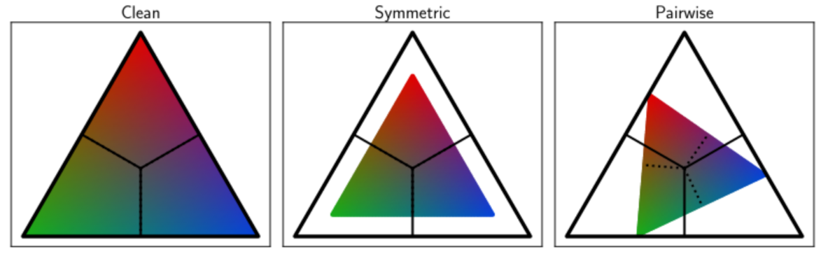
Ilustration of the noise tranisiton matrix as a linear transformation when working with 3 classes. The rescaling attempts to recover the original label distribution

From the confusion matrix, metrics and hence a cost function can be derived. Test.optimize tweaks the hyperparameters and carries a bayesian-optimization of the desired cost function. The bayesian optimizer deals better with computationally expensive evaluations of a sthocastic cost function, such in our case.

Practically, the above cited functions are members of the parent class Test. If your test is ready you only need to call them in order to get in return the optimal hyperparameters and the associated confusion matrix.

3. A Bayesian approach for merging multiple test evidences

We provide a function in order to deploy the test suite and merge the different results accounting the test performance achieved after optimisation. The vidences are merged through iterations of the bayes update rule.

For a set of N statistically independent tests:

$P(T_{i}|B)$ corresponds to the likelihood of an incorrect observation been flagged correctly. This is nothing but the confusion matrix estimated in the optimisation phase.

$P(B)$ corresponds to the prior probability that a given observation is incorrect. It is not trivial to estimate. In our case we estimate it from documents and calibration reports of the stations in our network. $P(B|T_{1},...,T_{N})$ corresponds to the posterior distribution, i.e probability that given a set of results issued by the suite of tests the observation is incorrect. This is the return value of our system.

multi_bayes loops over the pkl files in a give directory and creates the suite of tests for a given station returning an evaluation function which predicts the latter probability.

4. Visualisation and saving.

After optimisation and benchmarking, any test instance can be serialized to .pkl files and stored with their optimal hyperparameters and benchmarking information. Moreover, test_vis provides a nice and broad overview of the tests performance.

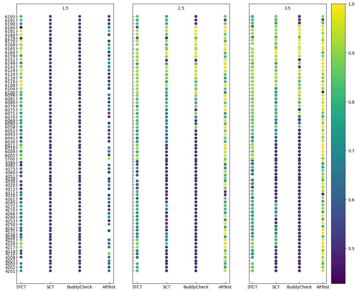
Example visualisation. Test accuracies after tuning. The Y-axis represents the stations ID. Variable: Temperature

Cite this work

If you used this package in your research and are interested in citing it here's how you do it:

@Misc{,
    author = {Tomás F. Bouvier},
    title = {Automatic detection of outliers in meteorological data},
    year = {2022},
    url = " https://github.com/tomasfbouvier/Meteorological_Data_quality_assesment"
}

Dependencies

• Numpy
• Scipy
• titanlib
• matplotlib
• pandas
• statsmodels

References

• https://github.com/metno/titanlib/wiki

• A Survey of Outlier Detection Methodologies.Victoria J. Hodge (vicky@cs.york.ac.uk) and Jim Austin

• A study on preprocessing and assimilation of Netatmo data in a NWP system, Alessandro Falcione

• Yang, X, K. S. Hintz, C. P. Aros and B. Amstrup, 2021, Danish Regional Atmospheric Reanalysis: Final scientific report of the 2020 NCKF Work Package 3.2.1, Regional Reanalysis Pilot. DMI report 21-31, 2021.

• Zhang et al., 2021, learning noise transition matrix from only noisy labels via total variation regularization

• Scott D. Anderson, 2007, Combining Evidence using Bayes' Rule